
IDEA StatiCa Detail – Constructief ontwerp van betonnen discontinuïteiten
De theoretische achtergrond is gebaseerd op COMPATIBLE STRESS FIELD DESIGN OF STRUCTURAL CONCRETE
(Kaufmann et al., 2020)
Constructief ontwerp van betonnen discontinuïteiten in IDEA StatiCa Detail
1 Inleiding tot de CSFM methode
1.1 Algemene inleiding voor het constructief ontwerp van betondetails
1.2 Belangrijkste aannames en beperkingen
1.3 Ontwerptools voor wapening
2 Analysemodel van IDEA StatiCa Detail
2.1 Inleiding tot de implementatie van eindige elementen
2.2 Opleggingen en belastingoverdrachtcomponenten
2.3 Belastingoverdracht bij afgesneden uiteinden van liggers
2.4 Geometrische aanpassing van doorsneden
2.5 Eindige elementen typen
2.6 Meshing
2.7 Oplossingsmethode en belastingsregelalgoritme
2.8 Presentatie van resultaten
3 Modelverificatie
3.1 Grentoestanden, scheurbreedteberekening en tension stiffening
4 Constructieve verificaties volgens EUROCODE
4.1 Materiaalmodellen (EN)
4.2 Veiligheidsfactoren
4.3 Analyse van de uiterste grenstoestand
4.4 Gedeeltelijk belaste oppervlakken (PLA)
4.5 Analyse van de bruikbaarheidsgrenstoestand
5 Constructieve verificaties volgens ACI 318-19
5.1 Materiaalmodellen (ACI)
5.2 Sterktereductie- en belastingsfactoren
5.3 Sterktecontroles
5.4 Opleggings- en verankeringszones - Gedeeltelijk belaste oppervlakken
5.5 Bruikbaarheidscontroles
6 Constructieve verificaties volgens AASHTO
6.1 Materiaalmodellen (AASHTO)
6.2 Weerstand- en belastingsfactoren
6.3 Sterktegrenstoestand
6.4 Weerstand van opleggings- en verankeringszones – Gedeeltelijk belaste oppervlakken
6.5 Gebruiksgrenstoestand
7 Constructieve verificaties volgens AS 3600
7.1 Materiaalmodellen (AUS)
7.2 Spanningsreductie- en belastingsfactoren
7.3 Sterkte- en verankeringscontroles
7.4 Bruikbaarheidscontroles
8 Voorspanning in Detail - Modelbeschrijving
1 Inleiding tot de CSFM methode
1.1 Algemene inleiding voor het constructief ontwerp van betondetails
Het ontwerp en de beoordeling van betonelementen worden normaal gesproken uitgevoerd op het niveau van de doorsnede (1D-element) of het punt (2D-element). Deze procedure is beschreven in alle normen voor constructief ontwerp, bijv. in (EN 1992-1-1 of ACI 318-19), en wordt dagelijks toegepast in de constructieve praktijk. Het is echter niet altijd bekend of gerespecteerd dat de procedure alleen acceptabel is in gebieden waar de Bernoulli-Navier hypothese van vlakke rekverdelingen van toepassing is (aangeduid als B-gebieden). De plaatsen waar deze hypothese niet van toepassing is, worden discontinuïteits- of verstoorde gebieden (D-gebieden) genoemd. Voorbeelden van B- en D-gebieden van 1D-elementen zijn weergegeven in (Fig. 1). Dit zijn bijvoorbeeld opleggingen, delen waar geconcentreerde belastingen worden aangebracht, locaties waar een abrupte verandering in de doorsnede optreedt, openingen, enz. Bij het ontwerpen van betonconstructies komen we ook veel andere D-gebieden tegen, zoals wanden, brugdiafragma's, consoles, enz.

\[ \textsf{\textit{\footnotesize{Fig. 1\qquad Discontinuity regions (Navrátil et al. 2017)}}}\]
In het verleden werden semi-empirische ontwerpregels gebruikt voor het dimensioneren van discontinuïteitsgebieden. Gelukkig zijn deze regels de afgelopen decennia grotendeels vervangen door staafwerkmodellen (Schlaich et al., 1987) en spanningsvelden (Marti 1985), die zijn opgenomen in de huidige ontwerpcodes en tegenwoordig veelvuldig door ontwerpers worden gebruikt. Deze modellen zijn mechanisch consistente en krachtige hulpmiddelen. Merk op dat spanningsvelden over het algemeen continu of discontinu kunnen zijn en dat staafwerkmodellen een speciaal geval zijn van discontinue spanningsvelden.
Ondanks de evolutie van rekentools in de afgelopen decennia worden Staafwerk-modellen in wezen nog steeds gebruikt als handberekeningen. Hun toepassing voor praktijkconstructies is omslachtig en tijdrovend, omdat iteraties vereist zijn en meerdere belastinggevallen in beschouwing moeten worden genomen. Bovendien is deze methode niet geschikt voor het verifiëren van bruikbaarheidscriteria (vervormingen, scheurbreedten, enz.).
De interesse van constructeurs in een betrouwbaar en snel hulpmiddel voor het ontwerpen van D-gebieden leidde tot de beslissing om de nieuwe Compatible Stress Field Method te ontwikkelen, een methode voor computerondersteund spanningsveldontwerp die het automatisch ontwerpen en beoordelen van constructief betonnen staven onder vlakke belasting mogelijk maakt.
De Compatible Stress Field Method (CSFM) is een continue op EEM gebaseerde spanningsveldanalysemethode waarbij klassieke spanningsveldoplossingen worden aangevuld met kinematische beschouwingen, d.w.z. de rekstoestand wordt door de gehele constructie geëvalueerd. Daardoor kan de effectieve druksterkte van beton automatisch worden berekend op basis van de dwarsrekstoestand, op een vergelijkbare manier als bij drukveldsanalyses die rekening houden met compression softening (Vecchio and Collins 1986; Kaufmann and Marti 1998) en de EPSF-methode (Fernández Ruiz and Muttoni 2007). Bovendien houdt de CSFM rekening met tension stiffening, waardoor realistische stijfheden aan de elementen worden toegekend, en dekt alle voorschriften uit de ontwerpcodes (inclusief bruikbaarheids- en vervormingscapaciteitsaspecten) die door eerdere benaderingen niet consistent werden behandeld. De CSFM maakt gebruik van gangbare eenassige spanning-rek-wetten die door ontwerpcodes worden voorgeschreven voor beton en wapening. Deze zijn bekend in de ontwerpfase, waardoor de partiële veiligheidsfactormethode kan worden toegepast. Ontwerpers hoeven daarom geen aanvullende, vaak willekeurige materiaaleigenschappen op te geven zoals doorgaans vereist bij niet-lineaire EEM-analyses, waardoor de methode perfect geschikt is voor de ingenieurspraktijk.
Om het gebruik van computerondersteunde spanningsvelden door constructeurs te bevorderen, dienen deze methoden te worden geïmplementeerd in gebruiksvriendelijke softwareomgevingen. Daartoe is de CSFM geïmplementeerd in IDEA StatiCa Detail; een nieuwe gebruiksvriendelijke commerciële software die gezamenlijk is ontwikkeld door ETH Zürich en het softwarebedrijf IDEA StatiCa in het kader van het DR-Design Eurostars-10571 project.
1.2 Belangrijkste aannames en beperkingen voor CSFM in 2D
CSFM beschouwt de maximale hoofdspanning in beton onder druk (σc2r) en wapenningsspanningen (σsr) ter plaatse van de scheuren, waarbij de treksterkte van het beton wordt verwaarloosd (σc1r = 0), met uitzondering van het stiffening effect op de wapening. De beschouwing van tension stiffening maakt het mogelijk de gemiddelde wapenningsrekken (εm) te simuleren. Er worden fictieve, roterende, spanningsvrije scheuren beschouwd die openen zonder glijding (Fig. 2a); tevens wordt rekening gehouden met het evenwicht ter plaatse van de scheuren en de gemiddelde rekken van de wapening.

\( \textsf{\textit{\footnotesize{Fig. 2\qquad Basic assumptions of the CSFM: (a) principal stresses in concrete; (b) stresses in the reinforcement direction;}}}\) \( \textsf{\textit{\footnotesize{(c) stress-strain diagram of concrete in terms of maximum stresses with consideration of compression softening;}}}\) \( \textsf{\textit{\footnotesize{(d) stress-strain diagram of reinforcement in terms of stresses at cracks and average strains; (e) compression softening}}}\) \( \textsf{\textit{\footnotesize{law; (f) bond shear stress-slip relationship for anchorage length verifications.}}}\)
Ondanks hun eenvoud is aangetoond dat vergelijkbare aannames nauwkeurige voorspellingen opleveren voor gewapende staven onder vlakke belasting (Kaufmann 1998; Kaufmann en Marti 1998), mits de aanwezige wapening brosse bezwijking bij scheurvorming voorkomt. Bovendien is het niet meenemen van enige bijdrage van de treksterkte van beton aan de uiterste belastingscapaciteit consistent met de beginselen van moderne ontwerpcodes, die grotendeels zijn gebaseerd op de plasticiteitstheorie.
Echter, de CSFM is niet geschikt voor slanke elementen zonder dwarswapening, omdat relevante mechanismen voor dergelijke elementen — zoals aggregaatgrijping, resterende trekspanningen aan de scheurpunt en deuvelwerking — die alle direct of indirect afhankelijk zijn van de treksterkte van het beton, worden verwaarloosd. Hoewel sommige ontwerpcodes het ontwerp van dergelijke elementen toestaan op basis van semi-empirische bepalingen, is de CSFM niet bedoeld voor dit type potentieel brosse constructies.
Beton
Het betonmodel dat in de CSFM is geïmplementeerd, is gebaseerd op de uniaxiale drukconstitutieve wetten die door ontwerpcodes zijn voorgeschreven voor het ontwerp van doorsneden, welke uitsluitend afhangen van de druksterkte. Het paraboolvormig-rechthoekig diagram (Fig. 2c) wordt standaard gebruikt in de CSFM, maar ontwerpers kunnen ook kiezen voor een meer vereenvoudigde elastisch-ideaal plastische relatie. Bij toetsing volgens de ACI-code kan uitsluitend het paraboolvormig-rechthoekig spanning-rek diagram worden gebruikt. Zoals eerder vermeld, wordt de treksterkte verwaarloosd, zoals ook het geval is bij klassiek gewapend betonontwerp.
De effectieve druksterkte wordt automatisch bepaald voor gescheurd beton op basis van de hoofdtrekrek (ε1) door middel van de reductiefactor kc2, zoals weergegeven in Fig. 2c en e. De geïmplementeerde reductieverhouding (Fig. 2e) is een generalisatie van het voorstel van de fib Model Code 2010 voor afschuivingstoetsingen, dat een grenswaarde van 0,65 bevat voor de maximale verhouding van effectieve betonsterkte tot betondruksterkte, welke niet van toepassing is op andere belastingssituaties.
De CSFM in IDEA StatiCa Detail beschouwt geen expliciet bezwijkcriterium in termen van rekken voor beton onder druk (d.w.z. er wordt een oneindig plastische tak beschouwd na het bereiken van de piekspanning). Deze vereenvoudiging maakt het niet mogelijk de vervormingscapaciteit te verifiëren van constructies die bezwijken onder druk. De uiterste capaciteit wordt echter correct voorspeld wanneer, naast de factor voor gescheurd beton (kc2) gedefinieerd in (Fig. 2e), de toename van de broosheid van beton bij toenemende sterkte in rekening wordt gebracht door middel van de reductiefactor \( \eta_{fc} \) zoals gedefinieerd in de fib Model Code 2010 als volgt:
\[f_{c,red} = k_c \cdot f_{c} = \eta _{fc} \cdot k_{c2} \cdot f_{c}\]
\[{\eta _{fc}} = {\left( {\frac{{30}}{{{f_{c}}}}} \right)^{\frac{1}{3}}} \le 1\]
waarbij:
kc de globale reductiefactor van de druksterkte is
kc2 de reductiefactor is als gevolg van de aanwezigheid van dwarsscheuren
fc de karakteristieke cilinderdruksterkte van het beton is (in MPa voor de definitie van \( \eta_{fc} \)).
Er is ook een reductie van de kc2 factor vanwege de stabiliteit van de berekening. Deze reductie heeft geen invloed op de totale sterkte van staven. Uitgaande van de waarde fcd als de gefactoriseerde sterkte van beton (rekenwaarde), wordt de waarde van kc2 gereduceerd volgens de volgende regels.
σc2r < 0.11fcd kc2=1.0
0.11fcd < σc2r < 0.37fcd kc2 is een lineaire interpolatie tussen 1,0 en de waarde afgelezen uit de
grafiek weergegeven in Fig. 2f
σc2r > 0.37fcd kc2 wordt direct afgelezen uit de grafiek van Fig. 2f
Wapening
Het geïdealiseerde bilineaire spanning-rek diagram voor onbedekte wapeningsstaven, zoals doorgaans gedefinieerd door ontwerpcodes (Fig. 2d), wordt beschouwd. De definitie van dit diagram vereist slechts kennis van de basiseigenschappen van de wapening tijdens de ontwerpfase (sterkte en duktiliteitsklasse). Een door de gebruiker gedefinieerde spanning-rek relatie kan ook worden ingevoerd.
Tension stiffening wordt verdisconteerd door de invoer spanning-rek relatie van de onbedekte wapeningsstaaf aan te passen, teneinde de gemiddelde stijfheid van de in het beton ingestorte staven te modelleren (εm).
Aanhechting model
Glijding tussen wapening en beton wordt in het eindige-elementenmodel geïntroduceerd door de vereenvoudigde star-volkomen plastische constitutieve relatie te beschouwen die is weergegeven in Fig. 2f, waarbij fbd de rekenwaarde (gefactoriseerde waarde) is van de maximale aanhechting zoals gespecificeerd door de ontwerpcode voor de specifieke aanhechtingsomstandigheden.
Dit is een vereenvoudigd model met als enig doel het verifiëren van aanhechtingsvoorschriften conform ontwerpcodes (d.w.z. verankering van wapening). De reductie van de verankeringslengte bij gebruik van haken, lussen en vergelijkbare staafvormen kan worden beschouwd door een bepaalde capaciteit te definiëren aan het uiteinde van de wapening, zoals hierna nader wordt beschreven.
1.3 Ontwerptools voor wapening
Workflow en doelstellingen
Het doel van de wapeningstoolsontwerp in de CSFM is om ontwerpers te helpen de locatie en de benodigde hoeveelheid wapeningsstaven efficiënt te bepalen. De volgende tools zijn beschikbaar om de gebruiker in dit proces te helpen/begeleiden: lineaire berekening en topologie-optimalisatie.
Wapeningstoolsontwerp maakt gebruik van vereenvoudigde constitutieve modellen in vergelijking met de modellen die worden gebruikt voor de definitieve verificatie van de constructie. Daarom moet de definitie van de wapening in deze stap worden beschouwd als een voorontwerp dat tijdens de definitieve verificatiestap bevestigd/verfijnd dient te worden. Het gebruik van de verschillende wapeningstoolsontwerp wordt geïllustreerd aan de hand van het model in Fig. 3, dat bestaat uit één uiteinde van een enkelvoudig opgelegde ligger met variabele hoogte, belast door een gelijkmatig verdeelde belasting.

\[ \textsf{\textit{\footnotesize{Fig. 3\qquad Model used to illustrate the use of the reinforcement design tools.}}}\]
Lineaire analyse
De lineaire analyse maakt gebruik van lineair elastische materiaaleigenschappen en verwaarloost de wapening in het betongebied. Het is daardoor een zeer snelle berekening die een eerste inzicht geeft in de locaties van trek- en drukgebieden. Een voorbeeld van een dergelijke berekening is weergegeven in Fig. 4.
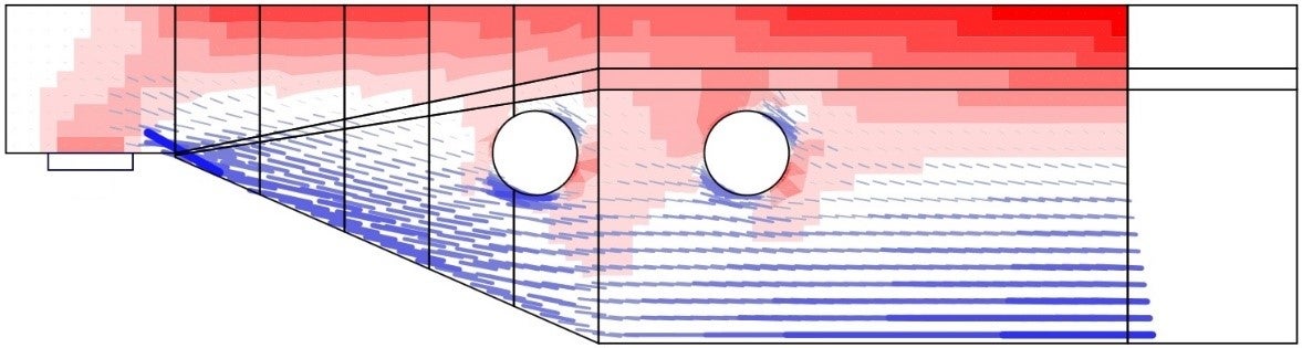
\[ \textsf{\textit{\footnotesize{Fig. 4\qquad Results from the linear analysis tool for defining reinforcement layout}}}\]
\[ \textsf{\textit{\footnotesize{(red: areas in compression, blue: areas in tension).}}}\]
Topologie-optimalisatie
Topologie-optimalisatie is een methode die tot doel heeft de optimale verdeling van materiaal in een gegeven volume te vinden voor een bepaalde belastingsconfiguratie. De topologie-optimalisatie die is geïmplementeerd in Idea StatiCa Detail maakt gebruik van een lineair eindige-elementenmodel. Elk eindig element kan een relatieve dichtheid hebben van 0 tot 100%, wat de relatieve hoeveelheid gebruikt materiaal vertegenwoordigt. Deze elementdichtheden zijn de optimalisatieparameters in het optimalisatieprobleem. De resulterende materiaaldistributie wordt als optimaal beschouwd voor de gegeven belastingscombinatie als deze de totale vervormingsenergie van het systeem minimaliseert. Per definitie is de optimale verdeling ook de geometrie met de grootst mogelijke stijfheid voor de gegeven belastingen.
Het iteratieve optimalisatieproces begint met een homogene dichtheidsverdeling. De berekening wordt uitgevoerd voor meerdere totale volumefracties (20%, 40%, 60% en 80%), waardoor de gebruiker het meest praktische resultaat kan selecteren. De resulterende vorm bestaat uit vakwerken met drukdiagonalen en trekstaven en vertegenwoordigt de optimale vorm voor de gegeven belastingscombinaties (Fig. 5).


\[ \textsf{\textit{\footnotesize{Fig. 5\qquad Results from the topology optimization design tool with 20\% and 40\% effective volume}}}\]
\[ \textsf{\textit{\footnotesize{(red: areas in compression, blue: areas in tension).}}}\]
2 Analysemodel van IDEA StatiCa Detail
2.1 Inleiding tot de implementatie van de Eindige Elementen Methode
De CSFM beschouwt continue spanningsvelden in het beton (2D eindige elementen), aangevuld met discrete "staaf"-elementen die de wapening vertegenwoordigen (1D eindige elementen). De wapening is dus niet diffuus ingebed in de 2D eindige elementen van het beton, maar expliciet gemodelleerd en hieraan gekoppeld. In het rekenmodel wordt een vlakke spanningstoestand beschouwd.

\[ \textsf{\textit{\footnotesize{Fig. 6\qquad Visualization of the calculation model of a structural element (trimmed beam) in Idea StatiCa Detail.}}}\]
Zowel volledige wanden als liggers, alsook details (delen) van liggers (geïsoleerd discontinuïteitsgebied, ook wel afgesneden uiteinde genoemd), kunnen worden gemodelleerd. Bij wanden en volledige liggers moeten de opleggingen zodanig worden gedefinieerd dat een (extern) isostatische (statisch bepaalde) of hyperstatische (statisch onbepaalde constructie) ontstaat. De krachtafdracht bij de afgesneden uiteinden van liggers wordt geïntroduceerd door middel van een speciale Saint-Venant overgangszone, die zorgt voor een realistische spanningsverdeling in het geanalyseerde detailgebied.
2.2 Ondersteuningen en lastoverdrachtende componenten
Om de meeste situaties tijdens het bouwproces te modelleren, zijn er in de CSFM veel soorten ondersteuningen (Fig. 7) en componenten voor lastoverdracht (Fig. 8) beschikbaar.
Ondersteuningen
Puntondersteuning kan op verschillende manieren worden gemodelleerd om te voorkomen dat spanningen in één punt worden geconcentreerd en in plaats daarvan over een groter gebied worden verdeeld. De eerste optie is een verdeelde puntondersteuning (Fig. 7a), die de belasting op de rand van de staaf gelijkmatig verdeelt over de opgegeven breedte.

\[ \textsf{\textit{\footnotesize{Fig. 7\qquad Various types of supports:}}}\]
\[ \textsf{\textit{\footnotesize{(a) point distributed; (b) bearing plate; (c) line support; (d) patch support; (e) hanging.}}}\]
Patch support (Fig. 7d) kan daarentegen alleen worden geplaatst binnen een betonvolume met een gedefinieerde effectieve straal. Het wordt vervolgens via stijve elementen verbonden met de knopen van het wapeningsnet binnen deze straal. Daarom is het vereist om een wapeningskooi rondom de patch support te definiëren.
Voor een nauwkeurigere modellering van bepaalde praktijksituaties zijn er twee andere opties voor puntondersteuning. Ten eerste is er puntondersteuning met een oplegplaat van gedefinieerde breedte en dikte (Fig. 7b). Het materiaal van de oplegplaat kan worden opgegeven en de volledige oplegplaat wordt onafhankelijk gemeshed. Ten tweede is er een hangende ondersteuning beschikbaar (Fig. 7e), die kan worden gebruikt voor het modelleren van hijsankers of hijsdeuvels.
Lijnondersteuning (Fig. 7c) kan worden gedefinieerd op een rand (door de lengte op te geven) of binnen een element (door een polylijn). Het is ook mogelijk om de stijfheid en/of het niet-lineaire gedrag te specificeren (ondersteuning in druk/trek of alleen in druk).
- Lees gedetailleerde beschrijvingen in Types of supports in IDEA StatiCa Detail
Lastoverdrachtende componenten
De introductie van belastingen in de constructie kan ook op verschillende manieren worden gemodelleerd. Voor puntlasten kan een oplegplaat (Fig. 8a) worden gebruikt, vergelijkbaar met puntondersteuning, waarbij de geconcentreerde belasting over een groter gebied wordt verdeeld dankzij een stalen plaat met gedefinieerde breedte en dikte.

\[ \textsf{\textit{\footnotesize{Fig. 8\qquad Various types of load transfer components:}}}\]
\[ \textsf{\textit{\footnotesize{(a) bearing plate; (b) patch load; (c) hanging; (d) partially loaded area.}}}\]
De puntlast kan direct op het oppervlak van de constructie worden aangebracht met een gedefinieerde werkingsstraal (de belasting wordt op de betonelementen aangebracht) of via een speciaal overdrachtsmechanisme genaamd patch load (Fig. 8b en Fig. 9). Patch load maakt het mogelijk de belasting direct over te dragen aan de gedefinieerde wapening binnen het gebied van de effectieve straal. Om de correcte werking van de patch load te waarborgen, is het noodzakelijk een groep staven te definiëren die worden verbonden met de belasting (in de wapeningseigenschappen). Wanneer de verbonden wapening niet is gedefinieerd, is het lastoverdrachtmechanisme hetzelfde als voor een puntlast op een staafoppervlak, en wordt de belasting via de randvoorwaarden overgedragen aan de betonelementen, niet direct aan de wapening.

\[ \textsf{\textit{\footnotesize{Fig. 9\qquad Patch load: (a) load application; (b) load transferred through rebars (a group of bars for the load transfer is defined);}}}\]
\[ \textsf{\textit{\footnotesize{(c) load transferred through concrete (a group of bars for the load transfer is not defined).}}}\]
Hijsankers of hijsdeuvels kunnen worden gemodelleerd door een hangende belasting (Fig. 8c). De gebruiker kan een gedeeltelijk belast gebied (Fig. 8d) toepassen, waarmee de draagkracht van beton onder druk kan worden verhoogd overeenkomstig de Eurocode (dit type lastoverdrachtend component kan niet worden gebruikt wanneer ACI is ingesteld). De constructie kan ook worden belast met lijnlasten op de randen, via een algemene polylijn of via oppervlaktelasten. De Detail applicatie kan automatisch het eigen gewicht in de berekening meenemen.
2.3 Krachtafdracht bij afgekotte uiteinden van balken
In veel gevallen hoeven we slechts een detail (deel) van een constructief element te modelleren, zoals een balkondersteuning, een opening in het midden van de balk, enz. Deze aanpak kan leiden tot ondersteuningsconfiguraties die onstabiel maar toelaatbaar zijn in IDEA StatiCa Detail (inclusief het geval zonder ondersteuningen). In dergelijke gevallen is het echter ook noodzakelijk om de doorsnede te modelleren die de verbinding met het aangrenzende B-gebied vertegenwoordigt, inclusief de inwendige krachten in deze doorsnede die aan de evenwichtsvoorwaarden voldoen. In bepaalde gevallen (bijv. bij het modelleren van een balkondersteuning) kunnen deze inwendige krachten automatisch door het programma worden bepaald.
Tussen het B-gebied en het geanalyseerde discontinuïteitsgebied wordt automatisch een Saint-Venant-overgangszone aangemaakt om een realistische spannningsverdeling in het geanalyseerde gebied te waarborgen. De breedte van de overgangszone wordt bepaald als de helft van de hoogte van de doorsnede. Omdat het enige doel van de Saint-Venant-zone is om een juiste spannningsverdeling in de rest van het model te bereiken, worden er geen resultaten uit dit gebied weergegeven bij de verificatie en worden hier geen stopcriteriagehanteerd.
De rand van de Saint-Venant-zone die het afgekotte uiteinde van de balk vertegenwoordigt, wordt gemodelleerd als stijf, d.w.z. deze mag roteren maar moet vlak blijven. Dit wordt gerealiseerd door alle FEM-knopen van de rand te verbinden met een afzonderlijke knoop in het traagheidscentrum van de doorsnede via een stijf lichaamselement (RBE2). De inwendige krachten van het element kunnen vervolgens worden aangebracht in deze knoop, zoals weergegeven in Fig. 10.

\[ \textsf{\textit{\footnotesize{Fig. 10\qquad Transfer of internal forces at a trimmed end.}}}\]
2.4 Geometrische aanpassing van doorsneden
Reductie van de doorsnede wordt automatisch uitgevoerd voor constructies die zijn gedefinieerd als een balk- of raamverbinding (gedefinieerd door de x-as en een doorsnede). Deze aanpassing wordt automatisch toegepast op doorsneden met zeer brede flenzen (Fig. 11) en is gebaseerd op de aanname dat een drukspanningsveld zich vanuit de wand uitbreidt onder een hoek van 45°, zodat de genoemde gereduceerde breedte de maximale breedte is die in staat is belastingen over te dragen.
Merk op dat de methode voor het bepalen van de effectieve flensbreedtte die in CSFM is geïmplementeerd, verschilt van de methode beschreven in 5.3.2.1 EN 1992-1-1 (2015) of in 9.2.4.4 ACI 318-19. Naast de geometrie wordt de op Eurocode gebaseerde effectieve flensbreedtte expliciet beïnvloed door de overspanningslengten en de randvoorwaarden van een constructie.

\[ \textsf{\textit{\footnotesize{Fig. 11\qquad Width reduction of a cross-section: (a) user input; (b) FE model – automatically determined reduced flange width.}}}\]
In het geval van consoles in het horizontale vlak (Fig. 12) wordt elke console verdeeld in vijf secties over de lengte. Elk van deze secties wordt vervolgens gemodelleerd als een wand met een constante dikte, die gelijk is aan de werkelijke dikte in het midden van de betreffende sectie.

\[ \textsf{\textit{\footnotesize{Fig. 12\qquad Horizontal haunch: (a) user input; (b) FE model – a haunch automatically divided into five sections.}}}\]
2.5 Eindige Elementen typen
Het niet-lineaire (inelastische) eindige elementenanalysemodel wordt opgebouwd uit verschillende typen eindige elementen die worden gebruikt om beton, wapening en de aanhechting daartussen te modelleren. Beton- en wapeningselementen worden eerst onafhankelijk van elkaar gemaild en vervolgens met elkaar verbonden via meerpuntsrandvoorwaarden (MPC-elementen). Hierdoor kan de wapening een willekeurige, relatieve positie ten opzichte van het beton innemen. Als de verificatie van de verankeringslengte moet worden berekend, worden bond- en veerelementen voor verankeringseinden ingevoegd tussen de wapening en de MPC-elementen.

\[ \textsf{\textit{\footnotesize{Fig. 13\qquad Finite element model: reinforcement elements mapped to concrete mesh using MPC elements and bond elements.}}}\]
Beton
Beton wordt gemodelleerd met vierhoekige en driehoekige schaalselementen, CQUAD4 en CTRIA3. Deze kunnen worden gedefinieerd door respectievelijk vier of drie knopen. In deze elementen wordt uitsluitend vlakke spanning verondersteld, d.w.z. spanningen of rekken in de z-richting worden niet beschouwd.
Elk element heeft vier of drie integratiepunten die op ongeveer 1/4 van de elementgrootte zijn geplaatst. In elk integratiepunt van elk element worden de richtingen van de hoofdrekken α1, α2 berekend. In beide richtingen worden de hoofdspanningen σc1, σc2 en de stijfheden E1, E2 bepaald op basis van het opgegeven spanning-rek diagram voor beton, zoals weergegeven in Fig. 2. Opgemerkt dient te worden dat het effect van compression softening het gedrag in de hoofddrukrichting koppelt aan de actuele toestand in de andere hoofdrichting.
Wapening
Wapeningsstaven worden gemodelleerd door twee-knoop 1D "staaf"-elementen (CROD), die uitsluitend axiale stijfheid bezitten. Deze elementen zijn verbonden met speciale "bond"-elementen die zijn ontwikkeld om het slipgedrag tussen een wapeningsstaf en het omringende beton te modelleren. Deze bond-elementen zijn vervolgens via MPC-elementen (meerpuntsrandvoorwaarden) verbonden met het mesh dat het beton vertegenwoordigt. Deze aanpak maakt onafhankelijke meshing van wapening en beton mogelijk, terwijl de onderlinge verbinding achteraf wordt gewaarborgd.
Bond-elementen
De verankeringslengte wordt geverifieerd door de bond-schuifspanningen tussen betonelementen (2D) en wapeningsstaafelementen (1D) in het eindige elementenmodel op te nemen. Hiertoe is een "bond" eindige-elementtype ontwikkeld.
De definitie van het bond-element is vergelijkbaar met die van een schaalelement (CQUAD4). Het wordt eveneens gedefinieerd door 4 knopen, maar in tegenstelling tot een schaal heeft het uitsluitend een niet-nul stijfheid in afschuiving tussen de twee bovenste en twee onderste knopen. In het model zijn de bovenste knopen verbonden met de elementen die de wapening vertegenwoordigen en de onderste knopen met die welke het beton vertegenwoordigen. Het gedrag van dit element wordt beschreven door de bondspanning, τb, als een bilineaire functie van de slip tussen de bovenste en onderste knopen, δu, zie Fig. 14.
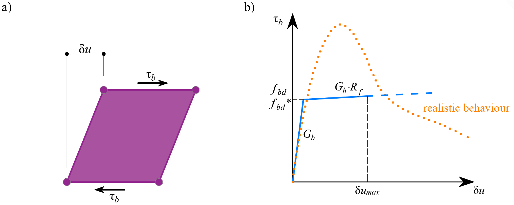
\[ \textsf{\textit{\footnotesize{Fig. 14\qquad (a) conceptual illustration of the deformation of a bond element; (b) a stress-deformation function.}}}\]
De elastische stijfheidsmodulus van de bond-slip relatie, Gb, wordt als volgt gedefinieerd:
\[G_b = k_g \cdot \frac{E_c}{Ø}\]
waarbij:
kg coëfficiënt afhankelijk van het oppervlak van de wapeningsstaf (standaard kg = 0,2)
Ec elasticiteitsmodulus van beton (aangenomen als Ecm in geval van EN)
Ø de diameter van de wapeningsstaf
De rekenwaarden (gecombineerde waarden) van de uiterste bond-schuifspanning, fbd, zoals vermeld in de respectievelijk geselecteerde normen EN 1992-1-1 of ACI 318-19, worden gebruikt voor de verificatie van de verankeringslengte. De verharding van de plastische tak wordt standaard berekend als Gb/105.
Verankeringsveer
Het aanbrengen van verankeringseinden aan de wapeningsstaven (d.w.z. bochten, haken, lussen…), die voldoen aan de voorschriften van de normen, maakt het mogelijk de basisverankeringslengte van de staven (lb,net) te reduceren met een bepaalde factor β (hierna aangeduid als de 'verankeringscoëfficiënt'). De rekenwaarde van de verankeringslengte (lb) wordt dan als volgt berekend:
\[l_b = \left(1 - \beta\right)l_{b,net}\]
De beoogde reductie van lb,net is equivalent aan de activering van de wapeningsstaf aan het uiteinde op een percentage van zijn maximale capaciteit, gegeven door de verankeringsreductiecoëfficiënt, zoals weergegeven in Fig. 15a.
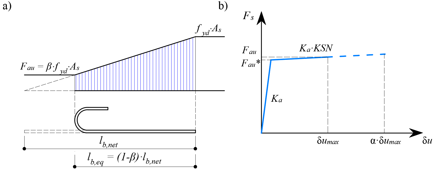
\[ \textsf{\textit{\footnotesize{Fig. 15\qquad Model for the reduction of the anchorage length:}}}\]
\[ \textsf{\textit{\footnotesize{(a) anchorage force along the anchorage length of the reinforcing bar; (b) slip-anchorage force constitutive relationship.}}}\]
De reductie van de verankeringslengte is opgenomen in het eindige elementenmodel door middel van een veerelement aan het uiteinde van de staaf (Fig. 15), dat wordt gedefinieerd door het constitutieve model weergegeven in Fig. 15b. De maximale kracht die door deze veer wordt overgedragen (Fau) is:
\[F_{au} = \beta \cdot A_s \cdot f_{yd}\]
waarbij:
β de verankeringscoëfficiënt op basis van het verankeringstype,
As de doorsnede van de wapeningsstaf,
fyd de rekenwaarde (gecombineerde waarde) van de vloeigrens van de wapening.
2.6 Mesh
De eindige elementen zijn intern geïmplementeerd en het analysemodel wordt automatisch gegenereerd zonder dat professionele gebruikersinteractie vereist is. Een belangrijk onderdeel van dit proces is de mesh.
Beton
Alle betonnen stavven worden samen gemeshed. Een aanbevolen elementgrootte wordt automatisch berekend door de applicatie op basis van de afmetingen en vorm van de constructie, rekening houdend met de diameter van de grootste wapeningsstaf. Bovendien garandeert de aanbevolen elementgrootte dat minimaal 4 elementen worden gegenereerd in dunne delen van de constructie, zoals slanke kolommen of dunne platen, om betrouwbare resultaten in deze gebieden te waarborgen. Het maximale aantal betonelementen is beperkt tot 5000, maar deze waarde is voldoende om de aanbevolen elementgrootte voor de meeste constructies te bieden. Ontwerpers kunnen altijd een door de gebruiker gedefinieerde betonelementsgrootte selecteren door de vermenigvuldiger van de standaard meshgrootte aan te passen.
Wapening
De wapening wordt verdeeld in elementen met ongeveer dezelfde lengte als de betonelementsgrootte. Zodra de wapenings- en betonmeshes zijn gegenereerd, worden ze onderling verbonden met aanhechtingselementen zoals weergegeven in Fig. 13.
Oplegplaten
Hulpconstructieve onderdelen, zoals oplegplaten, worden onafhankelijk gemeshed. De grootte van deze elementen wordt berekend als 2/3 van de grootte van betonelementen in het verbindingsgebied. De knopen van de oplegplaat-mesh worden vervolgens verbonden met de randknopen van de betonmesh via interpolatie-randvoorwaarde-elementen (RBE3).
Belastingen en opleggingen
Vlakbelastingen en vlaksteunpunten zijn alleen verbonden met de wapening, zoals weergegeven in Fig. 16. Daarom is het noodzakelijk om de wapening rondom deze te definiëren. Verbinding met alle knopen van de wapening binnen de effectieve straal wordt gewaarborgd door RBE3-elementen met gelijk gewicht.

\[ \textsf{\textit{\footnotesize{Fig. 16\qquad Patch load mapping to reinforcement mesh.}}}\]
Lijnsteunpunten en lijnbelastingen zijn verbonden met de knopen van de betonmesh via RBE3-elementen op basis van de opgegeven breedte of effectieve straal. Het gewicht van de verbindingen is omgekeerd evenredig met de afstand tot het steunpunt of de belastingsimpuls.
- Lees meer over de onderlinge verbinding tussen individuele belastingen en mesh in Algemene beschrijving van belastingsimpulsen in de Detail applicatie
2.7 Oplossingsmethode en belastingsbesturingsalgoritme
Een standaard volledig Newton-Raphson (NR) algoritme wordt gebruikt om de oplossing van een niet-lineair EEM-probleem te vinden.
Over het algemeen convergeert het NR-algoritme niet vaak wanneer de volledige belasting in één stap wordt opgelegd. Een gebruikelijke aanpak, die hier ook wordt toegepast, is om de belasting opeenvolgend in meerdere stappen op te leggen en het resultaat van de vorige belastingsstap te gebruiken als startpunt voor de Newton-oplossing van de volgende stap. Hiervoor is een belastingsbesturingsalgoritme geïmplementeerd bovenop de Newton-Raphson. In het geval dat de NR-iteraties niet convergeren, wordt de huidige belastingsstap gereduceerd tot de helft van zijn waarde, en worden de NR-iteraties opnieuw geprobeerd.
Een tweede doel van het belastingsbesturingsalgoritme is het vinden van de kritieke belasting, die overeenkomt met bepaalde "stopcriteriums" – specifiek de maximale rek in beton, de maximale slip in aanhechting-elementen, de maximale verplaatsing in verankeringselementen en de maximale rek in wapeningsstaven. De kritieke belasting wordt gevonden met behulp van de bisectiemethode. In het geval dat het stopcriterium ergens in het model wordt overschreden, worden de resultaten van de laatste belastingsstap verworpen en wordt een nieuwe stap van de helft van de vorige grootte berekend. Dit proces wordt herhaald totdat de kritieke belasting is gevonden met een bepaalde fouttolerantie.
Voor beton is het stopcriterium ingesteld op een rek van 5% bij druk (d.w.z. ongeveer een orde van grootte groter dan de werkelijke bezwijkrek van beton) en 7% bij trek in de integratiepunten van schaalelementen. Bij trek werd de waarde zo ingesteld dat de grensrek in de wapening, die gewoonlijk rond de 5% ligt zonder rekening te houden met tension stiffening, als eerste wordt bereikt. Bij druk werd de waarde gekozen uit meerdere alternatieven als een waarde die groot genoeg is zodat de effecten van verbrijzelen zichtbaar zijn in de resultaten, maar klein genoeg om niet te veel problemen met numerieke stabiliteit te veroorzaken.

\[ \textsf{\textit{\footnotesize{Fig. 17\qquad Constitutive relationship of bond and anchorage elements used for anchorage length verification:}}}\]
\[ \textsf{\textit{\footnotesize{(a) bond shear stress slip response of a bond element; (b) force-displacement response of an anchorage element.}}}\]
Voor wapening is het stopcriterium gedefinieerd in termen van spanningen. Omdat spanningen ter plaatse van de scheur worden gemodelleerd, komt het criterium bij trek overeen met de treksterkte van de wapening rekening houdend met de veiligheidscoëfficiënt. Dezelfde waarde wordt gebruikt voor het criterium bij druk.
Het stopcriterium in aanhechting-elementen en verankeringsveeren is α·δumax, waarbij δumax de maximale slip is die wordt gebruikt in normtoetsingen en α = 10.
2.8 Presentatie van resultaten
Resultaten worden afzonderlijk gepresenteerd voor beton en voor wapeningselementen. De spanning- en rekwaarden in beton worden berekend in de integratiepunten van schaalelementen. Omdat het echter niet praktisch is om de gegevens op deze manier te presenteren, worden de resultaten standaard gepresenteerd in knopen, zoals de maximale waarde van de drukspanning van aangrenzende Gauss-integratiepunten in verbonden elementen (Fig. 18). Opgemerkt dient te worden dat deze weergave de resultaten lokaal kan onderschatten aan de gedrukte randen van staven in het geval dat de eindige-elementgrootte vergelijkbaar is met de diepte van de drukzone.

Fig. 18 - Betonnen eindig element met integratiepunten en knopen: presentatie van de resultaten voor beton in knopen en in eindige elementen.
De resultaten voor de wapening eindige elementen zijn ofwel constant voor elk element (één waarde – bijv. voor staalspanningen) of lineair (twee waarden – voor aanhechting resultaten). Voor hulpelementen, zoals elementen van oplegplaten, worden alleen vervormingen gepresenteerd.
3 Modelverificatie
3.1 Grenstoestanden en scheurwijdteberekening
Beoordeling van de constructie met behulp van de CSFM wordt uitgevoerd door twee verschillende analyses: één voor bruikbaarheid en één voor belastingcombinaties in de uiterste grenstoestand. De bruikbaarheidsanalyse gaat ervan uit dat het uiterste gedrag van het element bevredigend is en dat de vloeigrensvoorwaarden van het materiaal niet worden bereikt bij bruikbaarheidsbelastingsniveaus. Deze aanpak maakt het gebruik van vereenvoudigde constitutieve modellen (met een lineaire tak van het spanning-rek diagram van beton) voor bruikbaarheidsanalyse mogelijk om de numerieke stabiliteit en berekeningssnelheid te verbeteren. Daarom wordt aanbevolen de hieronder gepresenteerde werkwijze te gebruiken, waarbij de analyse van de uiterste grenstoestand als eerste stap wordt uitgevoerd.
Analyse van de uiterste grenstoestand
De verschillende verificaties die vereist zijn door specifieke ontwerpcodes worden beoordeeld op basis van de directe resultaten van het model. UGT-verificaties worden uitgevoerd voor betonsterkte, wapeningssterkte en verankering (aanhechting schuifspanningen).
Om ervoor te zorgen dat een constructief element een efficiënt ontwerp heeft, wordt sterk aanbevolen een voorlopige analyse uit te voeren waarbij rekening wordt gehouden met de volgende stappen:
- Kies een selectie van de meest kritische belastingcombinaties.
- Bereken alleen belastingcombinaties in de Uiterste Grenstoestand (UGT).
- Gebruik een grof mesh (door de vermenigvuldiger van de standaard mesh-grootte in Setup te vergroten (Fig. 19)).

\[ \textsf{\textit{\footnotesize{Fig. 19\qquad Mesh multiplier.}}}\]
Een dergelijk model berekent zeer snel, waardoor ontwerpers de detaillering van het constructieve element efficiënt kunnen beoordelen en de analyse opnieuw kunnen uitvoeren totdat aan alle verificatievereisten is voldaan voor de meest kritische belastingcombinaties. Zodra aan alle verificatievereisten van deze voorlopige analyse is voldaan, wordt gesuggereerd de volledige uiterste belastingcombinaties op te nemen en een fijne mesh-grootte te gebruiken (de mesh-grootte aanbevolen door het programma). De gebruiker kan de mesh-grootte wijzigen via de vermenigvuldiger, die waarden kan bereiken van 0,5 tot 5 (Fig. 19).
De basisresultaten en verificaties (spanning, rek en benuttingsgraad (d.w.z. de berekende waarde/grenswaarde uit de norm), evenals de richting van de hoofdspanningen in het geval van betonelementen) worden weergegeven door middel van verschillende plots waarbij druk over het algemeen in rood en trek in blauw wordt weergegeven. Globale minimum- en maximumwaarden voor de gehele constructie kunnen worden gemarkeerd, evenals minimum- en maximumwaarden voor elk door de gebruiker gedefinieerd onderdeel. In een apart tabblad van het programma kunnen geavanceerde resultaten zoals tensorwaarden, vervormingen van de constructie en wapeningspercentages (effectief en geometrisch) die worden gebruikt voor het berekenen van de tension stiffening van wapeningsstaven worden weergegeven. Bovendien kunnen belastingen en reacties voor geselecteerde combinaties of belastinggevallen worden gepresenteerd.
Analyse van de bruikbaarheidsgrenstoestand
BGT-beoordelingen worden uitgevoerd voor spanningsbegrenzing, scheurwijdte en doorbuigingsgrenzen. Spanningen worden gecontroleerd in beton- en wapeningselementen overeenkomstig de toepasselijke norm op een vergelijkbare wijze als gespecificeerd voor de UGT.
De bruikbaarheidsanalyse bevat bepaalde vereenvoudigingen van de constitutieve modellen die worden gebruikt voor de analyse van de uiterste grenstoestand. Een perfecte aanhechting wordt verondersteld, d.w.z. de verankeringslengte wordt niet geverifieerd bij bruikbaarheid. Bovendien wordt de plastische tak van de spanning-rek curve van beton in druk buiten beschouwing gelaten, terwijl de elastische tak lineair en oneindig is. Deze vereenvoudigingen verbeteren de numerieke stabiliteit en berekeningssnelheid, en verminderen de algemeenheid van de oplossing niet zolang de resulterende materiaalspanningsgrenzen bij bruikbaarheid duidelijk onder hun vloeigrens liggen (zoals vereist door normen). Daarom zijn de vereenvoudigde modellen die worden gebruikt voor bruikbaarheid alleen geldig als aan alle verificatievereisten is voldaan.
Scheurwijdteberekening en tension stiffening
Scheurwijdteberekening
Er zijn twee manieren om scheurwijdten te berekenen: gestabiliseerde en niet-gestabiliseerde scheurvorming. Op basis van de geometrische wapeningsverhouding in elk deel van de constructie wordt bepaald welk type scheurberekeningsmodel wordt gebruikt (TCM voor gestabiliseerde scheurvorming en POM voor niet-gestabiliseerd scheurvorming model).

\( \textsf{\textit{\footnotesize{Fig. 20 \qquad Crack width calculation: (a) considered crack kinematics; (b) projection of crack kinematics into the principal}}}\) \( \textsf{\textit{\footnotesize{directions of the reinforcing bar; (c) crack width in the direction of the reinforcing bar for stabilized cracking; (d) cases with}}}\) \( \textsf{\textit{\footnotesize{local non-stabilized cracking regardless of the reinforcement amount; (e) crack width in the direction of the reinforcing bar}}}\)\( \textsf{\textit{\footnotesize{for non-stabilized cracking.}}}\)
Terwijl de CSFM voor de meeste verificaties een direct resultaat geeft (bijv. staafcapaciteit, doorbuigingen…), worden scheurwijdteresultaten berekend uit de wapeningsrekresultaten die rechtstreeks door de EE-analyse worden geleverd, volgens de methodologie beschreven in Fig. 20. Er wordt uitgegaan van een scheurkinematica zonder glijding (zuivere scheuropening) (Fig. 20a), wat consistent is met de belangrijkste aannames van het model. De hoofdrichtingen van spanningen en rekken bepalen de helling van de scheuren (θr = θs= θe). Volgens (Fig. 20b) kan de scheurwijdte (w) worden geprojecteerd in de richting van de wapeningsstaf (wb), wat leidt tot:
\[w = \frac{w_b}{\cos\left(θ_r + θ_b - \frac{π}{2}\right)}\]
waarbij θb de stafinclinate is.
Let op: het programma geeft waarden weer van θr en θb < π/2. Dit betekent dat de voorgaande vergelijking geldt voor gevallen waarbij de wapening en de scheur door verschillende kwadranten van het Cartesisch coördinatenstelsel lopen, zoals weergegeven in Fig. 20, waarbij de wapening door het I. en III. kwadrant loopt en de scheur door het II. en IV. kwadrant. Voor gevallen waarbij de wapening en de scheur door dezelfde kwadranten lopen, moet de vergelijking als volgt worden aangepast:
\[w = \frac{w_b}{\cos\left(-θ_r + θ_b + \frac{π}{2}\right)}\]
De component wb wordt consistent berekend op basis van de tension stiffening modellen door de wapeningsrekken te integreren. Voor die gebieden met volledig ontwikkelde scheurpatronen worden de berekende gemiddelde rekken (em) langs de wapeningsstaven direct geïntegreerd over de scheurafstand (sr), zoals aangegeven in (Fig. 20c). Hoewel deze benadering voor het berekenen van de scheurrichtingen niet overeenkomt met de werkelijke positie van de scheuren, levert zij toch representatieve waarden op die leiden tot scheurwijdteresultaten die kunnen worden vergeleken met de door de norm vereiste scheurwijdtewaarden ter plaatse van de wapeningsstaf.
Bijzondere situaties doen zich voor bij concave hoeken van de berekende constructie. In dit geval bepaalt de hoek de positie van een enkele scheur die zich op niet-gestabiliseerde wijze gedraagt voordat aangrenzende scheuren zich ontwikkelen. Deze aanvullende scheuren ontwikkelen zich over het algemeen na het bruikbaarheidsgebied (Mata-Falcón 2015), wat het rechtvaardigt om de scheurwijdten in een dergelijk gebied te berekenen alsof ze niet-gestabiliseerd zijn (Fig. 21).

\[ \textsf{\textit{\footnotesize{Fig. 21\qquad Definition of the region at concave corners in which the crack width is computed as if it were non-stabilized.}}}\]
Tension stiffening
De implementatie van tension stiffening maakt onderscheid tussen gevallen van gestabiliseerde en niet-gestabiliseerde scheurpatronen. In beide gevallen wordt het beton standaard als volledig gescheurd beschouwd vóór belasting.

\( \textsf{\textit{\footnotesize{Fig. 22\qquad Tension stiffening model: (a) tension chord element for stabilized cracking with distribution of bond shear,}}}\) \( \textsf{\textit{\footnotesize{steel and concrete stresses, and steel strains between cracks, considering average crack spacing); (b) pull-out assumption}}}\) \( \textsf{\textit{\footnotesize{for non-stabilized cracking with distribution of bond shear and steel stresses and strains around the crack; (c) resulting}}}\) \( \textsf{\textit{\footnotesize{tension chord behavior in terms of reinforcement stresses at the cracks and average strains for European B500B steel;}}}\) \( \textsf{\textit{\footnotesize{(d) detail of the initial branches of the tension chord response.}}}\)
Gestabiliseerde scheurvorming
Bij volledig ontwikkelde scheurpatronen wordt tension stiffening geïntroduceerd met behulp van het Tension Chord Model (TCM) (Marti et al. 1998; Alvarez 1998) – Fig. 22a – waarvan is aangetoond dat het uitstekende responsvoorspellingen oplevert ondanks zijn eenvoud (Burns 2012). Het TCM gaat uit van een getrapt, star-perfect plastisch aanhechting-schuifspanning-glijdingsverband met τb = τb0 =2 fctm voor σs ≤ fy en τb =τb1 = fctm voor σs > fy. Door elke wapeningsstaf als een trekkoord te beschouwen – Fig. 22b en Fig. 22a – kan de verdeling van de aanhechtingsschuifspanning, staal- en betonspanningen en daarmee de rekverdeling tussen twee scheuren worden bepaald voor elke gegeven waarde van de maximale staalspanningen (of rekken) ter plaatse van de scheuren.
Voor sr = sr0 kan al dan niet een nieuwe scheur ontstaan, omdat in het midden tussen twee scheuren σc1 = fct. Bijgevolg kan de scheurafstand variëren met een factor twee, d.w.z. sr = λsr0, met l = 0,5…1,0. Bij een bepaalde waarde voor λ kan de gemiddelde rek van het koord (εm) worden uitgedrukt als functie van de maximale wapeningsspanningen (d.w.z. spanningen ter plaatse van de scheuren, σsr). Voor het geïdealiseerde bilineaire spanning-rek diagram voor de wapeningsstaven dat standaard in de CSFM wordt gehanteerd, worden de volgende gesloten analytische uitdrukkingen verkregen (Marti et al. 1998):
\[\varepsilon_m = \frac{\sigma_{sr}}{E_s} - \frac{\tau_{b0}s_r}{E_s Ø}\]
\[\textrm{for}\qquad\qquad\sigma_{sr} \le f_y\]
\[{\varepsilon_m} = \frac{{{{\left( {{\sigma_{sr}} - {f_y}} \right)}^2}Ø}}{{4{E_{sh}}{\tau _{b1}}{s_r}}}\left( {1 - \frac{{{E_{sh}}{\tau_{b0}}}}{{{E_s}{\tau_{b1}}}}} \right) + \frac{{\left( {{\sigma_{sr}} - {f_y}} \right)}}{{{E_s}}}\frac{{{\tau_{b0}}}}{{{\tau_{b1}}}} + \left( {{\varepsilon_y} - \frac{{{\tau_{b0}}{s_r}}}{{{E_s}Ø}}} \right)\]
\[\textrm{for}\qquad\qquad{f_y} \le {\sigma _{sr}} \le \left( {{f_y} + \frac{{2{\tau _{b1}}{s_r}}}{Ø}} \right)\]
\[ \varepsilon_m = \frac{f_s}{E_s} + \frac{\sigma_{sr}-f_y}{E_{sh}} - \frac{\tau_{b1} s_r}{E_{sh} Ø}\]
\[\textrm{for}\qquad\qquad\left(f_y + \frac{2\tau_{b1}s_r}{Ø}\right) \le \sigma_{sr} \le f_t\]
waarbij:
Esh de staalverhardingsmodulus Esh = (ft – fy)/(εu – fy /Es) ,
Es elasticiteitsmodulus van de wapening,
Ø diameter van de wapeningsstaf,
sr scheurafstand,
σsr wapeningsspanningen ter plaatse van de scheuren,
σs actuele wapeningsspanningen,
fy vloeigrens van de wapening.
De Idea StatiCa Detail implementatie van de CSFM houdt standaard rekening met de gemiddelde scheurafstand bij het uitvoeren van computerondersteunde spanningsveldanalyse. De gemiddelde scheurafstand wordt beschouwd als 2/3 van de maximale scheurafstand (λ = 0,67), wat aansluit bij aanbevelingen op basis van buigings- en trekproeven (Broms 1965; Beeby 1979; Meier 1983). Opgemerkt dient te worden dat bij de berekening van scheurwijdten een maximale scheurafstand (λ = 1,0) wordt gehanteerd om conservatieve waarden te verkrijgen.
De toepassing van het TCM is afhankelijk van de wapeningsverhouding, en daarom is de toewijzing van een geschikte betonoppervlakte die tussen de scheuren op trek werkt aan elke wapeningsstaf cruciaal. Er is een automatische numerieke procedure ontwikkeld om de bijbehorende effectieve wapeningsverhouding (ρeff = As/Ac,eff) voor elke configuratie, inclusief schuine wapening (Fig. 23).

\( \textsf{\textit{\footnotesize{Fig. 23\qquad Effective area of concrete in tension for stabilized cracking: (a) maximum concrete area that can be activated;}}}\) \( \textsf{\textit{\footnotesize{(b) cover and global symmetry condition; (c) resultant effective area.}}}\)
Niet-gestabiliseerde scheurvorming
Scheuren in gebieden met geometrische wapeningsverhoudingen lager dan ρcr, d.w.z. de minimale hoeveelheid wapening waarbij de wapening in staat is de scheurlast op te nemen zonder te vloeien, worden veroorzaakt door niet-mechanische invloeden (bijv. krimp) of door de voortgang van scheuren die worden beheerst door andere wapening. De waarde van deze minimale wapening wordt als volgt bepaald:
\[{\rho _{cr}} = \frac{{{f_{ct}}}}{{{f_y} - \left( {n - 1} \right){f_{ct}}}}\]
waarbij:
fy vloeigrens van de wapening,
fct treksterkte van het beton,
n modulaire verhouding, n = Es / Ec .
Voor gangbaar beton en wapeningsstaal bedraagt ρcr ongeveer 0,6%.
Voor beugels met wapeningsverhoudingen onder ρcr wordt scheurvorming als niet-gestabiliseerd beschouwd en wordt tension stiffening geïmplementeerd door middel van het Pull-Out Model (POM) beschreven in Fig. 22b. Dit model analyseert het gedrag van een enkele scheur zonder mechanische interactie tussen afzonderlijke scheuren, waarbij de vervormingscapaciteit van het beton op trek wordt verwaarloosd en dezelfde getrapte, star-perfect plastische aanhechtingsschuifspanning-glijdingsrelatie wordt aangenomen als gebruikt door het TCM. Dit maakt het mogelijk om de wapeningsrekverdeling (εs) in de nabijheid van de scheur te bepalen voor elke maximale staalspanning ter plaatse van de scheur (σsr) rechtstreeks uit evenwicht. Gezien het feit dat de scheurafstand onbekend is bij een niet-volledig ontwikkeld scheurpatroon, wordt de gemiddelde rek (εm) berekend voor elk belastingsniveau over de afstand tussen punten met nulglijding wanneer de wapeningsstaf zijn treksterkte (ft) bereikt ter plaatse van de scheur (lε,avg in Fig. 22b), wat leidt tot de volgende betrekkingen:

De voorgestelde modellen maken de berekening mogelijk van het gedrag van verankerde wapening, dat uiteindelijk in de analyse wordt meegenomen. Dit gedrag (inclusief tension stiffening) voor het meest gangbare Europese wapeningsstaal (B500B, met ft / fy = 1,08 en εu = 5%) is weergegeven in Fig. 22c-d.
4 Constructieve verificaties volgens Eurocode
De beoordeling van de constructie met behulp van CSFM wordt uitgevoerd door twee verschillende analyses: één voor de bruikbaarheidsgrenstoestand en één voor de uiterste grenstoestand belastingcombinaties. De bruikbaarheidsanalyse gaat ervan uit dat het uiterste gedrag van het element bevredigend is en dat de vloeigrens van het materiaal niet wordt bereikt bij bruikbaarheidsbelastingsniveaus. Deze aanpak maakt het gebruik van vereenvoudigde constitutieve modellen (met een lineaire tak van het spanning-rek diagram van beton) voor de bruikbaarheidsanalyse mogelijk om de numerieke stabiliteit en berekeningssnelheid te verbeteren.
4.1 Materiaalmodellen (EN)
Beton - UGT
Het betonmodel dat is geïmplementeerd in de CSFM is gebaseerd op de eenassige druk constitutieve wetten voorgeschreven door EN 1992-1-1 voor het ontwerp van doorsneden, die alleen afhangen van de druksterkte. Het paraboolvormig-rechthoekig diagram gespecificeerd in EN 1992-1-1 Cl. 3.1.7 (1) (Fig. 24a) wordt standaard gebruikt in de CSFM, maar ontwerpers kunnen ook kiezen voor een meer vereenvoudigde elastisch ideaal plastische relatie volgens EN 1992-1-1 Cl. 3.1.7 (2) (Fig. 24b). De treksterkte wordt verwaarloosd, zoals ook het geval is in het klassieke gewapend betonontwerp.

\[ \textsf{\textit{\footnotesize{Fig. 24\qquad De spanning-rek diagrammen van beton voor UGT: a) paraboolvormig-rechthoekig diagram; b) bilineair diagram.}}}\]
De implementatie van de CSFM in IDEA StatiCa Detail houdt geen rekening met een expliciet bezwijkcriterium in termen van rekken voor beton onder druk (d.w.z. na het bereiken van de piekspanning wordt een plastische tak beschouwd met εcu2 (εcu3) met een waarde van 5%, terwijl EN 1992-1-1 een uiterste rek van minder dan 0,35% aanneemt). Deze vereenvoudiging maakt het niet mogelijk om de vervormingscapaciteit te verifiëren van constructies die bezwijken onder druk. De uiterste capaciteit fcd volgens EN 1992-1-1 3.1.3 wordt echter correct voorspeld wanneer, naast de factor voor gescheurd beton (kc2 gedefinieerd in (Fig. 25)), de toename van de broosheid van beton naarmate de sterkte stijgt in aanmerking wordt genomen door middel van de \(\eta_{fc}\) reductiefactor gedefinieerd in fib Model Code 2010 als volgt:
\[f_{cd}={\alpha_{cc}} \cdot \frac{f_{ck,red}}{γ_c} = {\alpha_{cc}} \cdot \frac{k_c \cdot f_{ck}}{γ_c} = {\alpha_{cc}} \cdot \frac{\eta _{fc} \cdot k_{c2} \cdot f_{ck}}{γ_c}\]
\[{\eta _{fc}} = {\left( {\frac{{30}}{{{f_{ck}}}}} \right)^{\frac{1}{3}}} \le 1\]
waarbij:
αcc is de coëfficiënt die rekening houdt met langetermijneffecten op de druksterkte en met ongunstige effecten als gevolg van de wijze waarop de belasting wordt aangebracht. Deze is conform EN 1992-1-1 Cl. 3.1.6 (1). De standaardwaarde is 1,0.
kc is de globale reductiefactor van de druksterkte
kc2 is de reductiefactor als gevolg van de aanwezigheid van dwarsscheuren
fck is de karakteristieke cilinderdruksterkte van beton (in MPa voor de definitie van \( \eta_{fc} \)).

\[ \textsf{\textit{\footnotesize{Fig. 25\qquad De compression softening wet.}}}\]
Beton - BGT
De bruikbaarheidsanalyse bevat bepaalde vereenvoudigingen van de constitutieve modellen die worden gebruikt voor de analyse van de uiterste grenstoestand. De plastische tak van de spanning-rek curve van beton onder druk wordt buiten beschouwing gelaten, terwijl de elastische tak lineair en oneindig is. De compression softening wet wordt niet beschouwd. Deze vereenvoudigingen verbeteren de numerieke stabiliteit en de berekeningssnelheid en verminderen de algemeenheid van de oplossing niet, zolang de resulterende materiaalspanningsgrenzen bij bruikbaarheid duidelijk onder hun vloeipunten liggen (zoals vereist door de Eurocode). Daarom zijn de vereenvoudigde modellen die worden gebruikt voor bruikbaarheid alleen geldig als aan alle verificatievereisten is voldaan.

\[ \textsf{\textit{\footnotesize{Fig. 26\qquad Spanning-rek diagrammen van beton geïmplementeerd voor bruikbaarheidsanalyse: korte- en langetermijnverificaties.}}}\]
Langetermijneffecten
Bij de bruikbaarheidsanalyse worden de langetermijneffecten van beton beschouwd met behulp van een effectieve oneindige kruipcoëfficiënt (\(\varphi\), standaard ingesteld op 2,5) die de secansmodulus van elasticiteit van beton (Ecm) aanpast conform EN 1992-1-1, paragraaf 3.1.4 (3) resp. 7.4.3 (5) als volgt:
\[E_{c,eff} = \frac{E_{cm}}{1+\varphi}\]
Bij het beschouwen van langetermijneffecten wordt eerst een belastingstap met alle permanente belastingen berekend met de kruipcoëfficiënt (d.w.z. met de effectieve elasticiteitsmodulus van beton, Ec,eff), waarna de aanvullende belastingen worden berekend zonder de kruipcoëfficiënt (d.w.z. met Ecm). Daarnaast wordt voor kortetermijnverificaties een aparte berekening uitgevoerd waarbij alle belastingen worden berekend zonder de kruipcoëfficiënt. Beide berekeningen voor lange- en kortetermijnverificaties zijn weergegeven in Fig. 26.
Kruipfactoren worden door de gebruiker gedefinieerd in de materiaaleigenschappen en dienen te worden berekend conform EN 1992-1-1, Fig. 3.1.
Wapening
Standaard wordt het geïdealiseerde bilineaire spanning-rek diagram voor onbedekte wapeningsstaven gedefinieerd in EN 1992-1-1, paragraaf 3.2.7 (Fig. 27) beschouwd. De definitie van dit diagram vereist alleen dat de basiseigenschappen van de wapening bekend zijn tijdens de ontwerpfase (sterkte en duktiliteitsklasse). Wanneer bekend, kan de werkelijke spanning-rek relatie van de wapening (warmgewalst, koudbewerkt, geblust en zelfontlaten, …) worden beschouwd. Het spanning-rek diagram van de wapening kan door de gebruiker worden gedefinieerd, maar in dat geval is het niet mogelijk om het tension stiffening effect aan te nemen (het is niet mogelijk om de scheurwijdte te berekenen). Het gebruik van het spanning-rek diagram met een horizontale bovenste tak maakt verificatie van de constructieve duurzaamheid niet mogelijk. Daarom is handmatige verificatie van de standaard duktiliteitseisen noodzakelijk.

\( \textsf{\textit{\footnotesize{Fig. 27 \qquad Spanning-rek diagram van wapening: a) bilineair diagram met een hellende bovenste tak; b) bilineair diagram}}}\) \( \textsf{\textit{\footnotesize{met een horizontale bovenste tak.}}}\)
Tension stiffening (Fig. 28) wordt automatisch in rekening gebracht door de invoer spanning-rek relatie van de onbedekte wapeningsstaaf aan te passen om de gemiddelde stijfheid van de in beton ingestorte staven te beschrijven (εm).

\[ \textsf{\textit{\footnotesize{Fig. 28\qquad Schema van tension stiffening.}}}\]
4.2 Veiligheidsfactoren
De Compatible Stress Field Method voldoet aan moderne ontwerpcodes. Omdat de rekenmodellen uitsluitend standaard materiaaleigenschappen gebruiken, kan het partiële veiligheidsfactorenformaat dat in de ontwerpcodes is voorgeschreven zonder aanpassing worden toegepast. Op deze manier worden de invoerbelastingen gefactoriseerd en worden de karakteristieke materiaaleigenschappen gereduceerd met behulp van de respectieve veiligheidscoëfficiënten die in de ontwerpcodes zijn voorgeschreven, precies zoals bij conventionele betonanalyse. Waarden van materiaalveiligheidsfactoren voorgeschreven in EN 1992-1-1 hfdst. 2.4.2.4 zijn standaard ingesteld, maar de gebruiker kan veiligheidsfactoren wijzigen in de Code- en berekeningsinstellingen (Fig. 29).
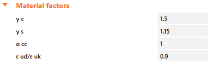
\[ \textsf{\textit{\footnotesize{Fig. 29\qquad The setting of material safety factors in Idea StatiCa Detail.}}}\]
Belastingsveiligheidsfactoren moeten door de gebruiker worden gedefinieerd in Combinatieregels voor elke niet-lineaire combinatie van belastinggevallen (Fig. 30). Voor alle templates die zijn geïmplementeerd in Idea StatiCa Detail, zijn partiële veiligheidsfactoren reeds voorgedefinieerd.
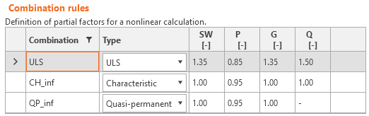
\[ \textsf{\textit{\footnotesize{Fig. 30\qquad The setting of load partial factors in Idea StatiCa Detail.}}}\]
Door gebruik te maken van door de gebruiker gedefinieerde combinaties van partiële veiligheidsfactoren kunnen gebruikers ook berekeningen uitvoeren met de CSFM via de globale weerstandsfactormethode (Navrátil, et al. 2017), maar deze aanpak wordt in de ontwerppraktijk nauwelijks gebruikt. Sommige richtlijnen bevelen het gebruik van de globale weerstandsfactormethode aan voor niet-lineaire analyse. Bij vereenvoudigde niet-lineaire analyses (zoals de CSFM), waarbij alleen die materiaaleigenschappen vereist zijn die ook bij conventionele handberekeningen worden gebruikt, verdient het partiële veiligheidsformaat echter nog steeds de voorkeur.
4.3 Analyse van de uiterste grenstoestand
De verschillende verificaties die vereist zijn door EN 1992-1-1 worden beoordeeld op basis van de directe resultaten van het model. UGT-verificaties worden uitgevoerd voor betonsterkte, wapeningststerkte en verankering (aanhechting schuifspanningen).
De betonsterkte bij druk wordt beoordeeld als de verhouding tussen de maximale hoofddrukspanning σc = σc2 verkregen uit de EEM-analyse en de grenswaarde σc,lim = fcd.
De sterkte van de wapening wordt beoordeeld bij zowel trek als druk als de verhouding tussen de spanning in de wapening ter plaatse van de scheuren σsr en de opgegeven grenswaarde σs,lim:
\(σ_{s,lim} = \frac{k \cdot f_{yk}}{γ_s}\qquad\qquad\textsf{\small{for bilinear diagram with inclined top branch}}\)
\(σ_{s,lim} = \frac{f_{yk}}{γ_s}\qquad\qquad\,\,\,\,\textsf{\small{for bilinear diagram with horizontal top branch}}\)
waarbij:
fyk vloeigrens van de wapening volgens EN 1992-1-1 Art. 3.2.3,
k de verhouding van de treksterkte ftk tot de vloeigrens,
\(k = \frac{f_{tk}}{f_{yk}}\)
γs is de partiële veiligheidsfactor voor wapening
De aanhechting schuifspanning wordt afzonderlijk beoordeeld als de verhouding tussen de aanhechtingsspanning τb berekend door de EEM-analyse en de uiterste aanhechtingssterkte fbd, volgens EN 1992-1-1 par. 8.4.2:
\[\frac{τ_{b}}{f_{bd}}\]
\[f_{bd} = 2.25 \cdot η_1\cdot η_2\cdot f_{ctd}\]
waarbij:
fctd is de rekenwaarde van de betonnen treksterkte volgens EN 1992-1-1 Art. 3.1.6 (2). Vanwege de toenemende broosheid van hogersterk beton is fctk,0.05 beperkt tot de waarde voor C60/75 volgens EN 1992-1-1 Art. 8.4.2 (2)
η1 is een coëfficiënt gerelateerd aan de kwaliteit van de aanhechtingsomstandigheden en de positie van de staaf tijdens het betonnen (Fig. 31).
η1 = 1,0 wanneer 'goede' omstandigheden worden verkregen en
η1 = 0,7 voor alle andere gevallen en voor staven in constructieve elementen gebouwd met glijbekisting, tenzij aangetoond kan worden dat 'goede' aanhechtingsomstandigheden bestaan
η2 is gerelateerd aan de staafdiameter:
η2 = 1,0 voor Ø ≤ 32 mm
η2 = (132 - Ø)/100 voor Ø > 32 mm

\[ \textsf{\textit{\footnotesize{Fig. 31\qquad EN 1992-1-1 Figure 8.2 - Description of bond conditions.}}}\]
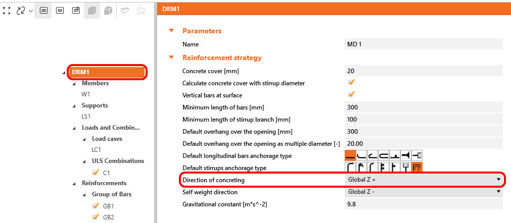
In IDEA StatiCa Detail worden de aanhechtingsomstandigheden in aanmerking genomen volgens Fig. 31 c) en d). De betonneerrichting kan in de applicatie voor elk projectonderdeel als volgt worden ingesteld.
Deze verificaties worden uitgevoerd met betrekking tot de toepasselijke grenswaarden voor de respectieve delen van de constructie (d.w.z. ondanks het gebruik van één kwaliteit voor zowel beton- als wapeningstmateriaal, zullen de uiteindelijke spanning-rek diagrammen in elk deel van de constructie verschillen vanwege tension stiffening en compression softening effecten).
Er is ook een optie om gladde staven te modelleren. Meer informatie is hier te vinden: Gladde staven in Detail
Totale kracht Ftot en grenskracht Flim
De totale kracht Ftot is een resultaat van de eindige elementenanalyse en kan op twee manieren worden gedefinieerd.
\[F_{tot}=A_{s}\cdot \sigma_{s}\]
waarbij As de oppervlakte van de wapeningsstaaf is en σs de spanning in de staaf is.
Of als de som van de verankeringskracht Fa en de aanhechtingskracht Fbond.
\[F_{tot}=F_{a}+F_{bond}\]
waarbij Fa de werkelijke kracht in de verankeringsveer is en Fbond de aanhechtingskracht is die verkregen kan worden door de aanhechtingsspanning τb te integreren over de lengte van de wapeningsstaaf l.
\[F_{bond}=C_{s} \cdot \int_{0}^{l}\tau_{b}\left( x \right)dx\]
Cs is de omtrek van de wapeningsstaaf.
De grenskracht Flim is de maximale kracht in het element van de wapeningsstaaf, rekening houdend met de uiterste sterkte van de staaf en ook de verankeringsomstandigheden (aanhechting tussen beton en wapening en verankeringshaken, lussen, enz.).
\[F_{lim}=min\left( F_{lim,bond}+F_{au},F_{u} \right)\]
\[F_{u}=k\cdot f_{yd}\cdot A_{s}\]
\[F_{au}=\beta\cdot k\cdot f_{yd}\cdot A_{s}\]
\[F_{lim,bond}=C_{s}\cdot l \cdot f_{bd}\]
waarbij Cs de omtrek van de wapeningsstaaf is en l de lengte is vanaf het begin van de wapeningsstaaf tot het beschouwde punt.

\[ \textsf{\textit{\footnotesize{Fig. 32\qquad Definition of the limit force Flim}}}\]
\[F_{lim,2}=F_{lim,1}+F_{lim,add}\]
waarbij Flim,add de aanvullende kracht is berekend uit de grootte van de hoek tussen naburige elementen. Flim,2 moet altijd kleiner zijn dan Fu.
De beschikbare verankeringstypen in de CSFM omvatten een rechte staaf (d.w.z. geen reductie van het verankeringsgedeelte), buiging, haak, lus, gelaste dwarsstang, perfecte aanhechting en doorgaande staaf. Al deze typen, samen met de respectieve verankeringscoëfficiënten β, zijn weergegeven in Fig. 32 voor langswapening en in Fig. 33 voor beugels. De waarden van de gehanteerde verankeringscoëfficiënten zijn in overeenstemming met EN 1992-1-1 paragraaf 8.4.4 Tab. 8.2. Opgemerkt dient te worden dat ondanks de verschillende beschikbare opties, de CSFM drie typen verankeringseinden onderscheidt: (i) geen reductie van de verankeringslengte, (ii) een reductie van 30% van de verankeringslengte bij een genormaliseerde verankering en (iii) perfecte aanhechting.

\[ \textsf{\textit{\footnotesize{Fig. 33\qquad Available anchorage types and respective anchorage coefficients for longitudinal reinforcing bars in the CSFM:}}}\]
\[ \textsf{\textit{\footnotesize{(a) straight bar; (b) bend; (c) hook; (d) loop; (e) welded transverse bar; (f) perfect bond; (g) continuous bar.}}}\]
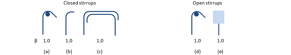
\[ \textsf{\textit{\footnotesize{Fig. 33\qquad Available anchorage types and respective anchorage coefficients for stirrups.}}}\]
\[ \textsf{\textit{\footnotesize{Closed stirrups: (a) hook; (b) bend; (c) overlap. Open stirrups: (d) hook; (e) continuous bar.}}}\]
Om te voldoen aan EN 1992-1-1 dient de verankeringsveer in de berekening te worden gebruikt; de verankeringsveer wordt aangepast door de β-coëfficiënt, zodat de gebruiker een van de beschikbare verankeringstypen moet gebruiken bij het definiëren van de begin- en eindcondities van de wapening.
4.4 Gedeeltelijk belaste gebieden (PLA)
Bij het ontwerpen van betonconstructies komen we twee grote groepen gedeeltelijk belaste gebieden (PLA) tegen - de eerste groep omvat opleggingen, terwijl de andere bestaat uit verankeringsgebieden. Volgens de momenteel geldende normen voor het ontwerp van gewapend betonconstructies EN 1992-1-1 hfdst. 6.7 (Fig. 34), dient rekening te worden gehouden met lokaal verbrijzelen van het beton en dwarse trekkrachten voor gedeeltelijk belaste gebieden. Voor een gelijkmatig verdeelde belasting op een oppervlak Ac0, kan de drukweerstand van beton worden verhoogd tot driemaal, afhankelijk van het rekenmatige verdelingsoppervlak Ac1.

\[ \textsf{\textit{\footnotesize{Fig. 34\qquad Partially loaded areas according to EN 1992-1-1.}}}\]
Het gedeeltelijk belaste gebied moet voldoende worden bewapend met dwarse wapening die is ontworpen om de scheurende krachten over te dragen die in het gebied optreden. Voor het ontwerp van dwarse wapening in gedeeltelijk belaste gebieden wordt de Staafwerk-methode gebruikt conform de Eurocode. Zonder de vereiste dwarse wapening is het niet mogelijk om de verhoogde drukweerstand van het beton in rekening te brengen.
Gedeeltelijk belaste gebieden in de CSFM

\[ \textsf{\textit{\footnotesize{Fig. 35\qquad Fictitious struts with concrete finite element mesh.}}}\]
Met behulp van de CSFM is het mogelijk om gewapend betonconstructies te ontwerpen en te beoordelen, inclusief de invloed van de toenemende drukweerstand van beton in gedeeltelijk belaste gebieden. Omdat de CSFM een wand (2D) model is en de gedeeltelijk belaste gebieden een ruimtelijke (3D) opgave zijn, was het noodzakelijk een oplossing te vinden die deze twee verschillende typen opgaven combineert (Fig. 35). Als de functie "gedeeltelijk belaste gebieden" is geactiveerd, wordt de toelaatbare kegelgeometrie aangemaakt conform de Eurocode (Fig. 34). Alle geometrische conflicten worden volledig in 3D opgelost voor de opgegeven betonstaaf-geometrie en de afmetingen van elke PLA. Vervolgens wordt een rekenmodel van het gedeeltelijk belaste gebied aangemaakt.

\[ \textsf{\textit{\footnotesize{Fig. 36\qquad Allowable cone geometries.}}}\]
De aanpassing van het materiaalmodel bleek een ongeschikte aanpak te zijn, voornamelijk omdat het toewijzen van eigenschappen aan de eindige elementen mesh problematisch is. Er werd vastgesteld dat een aanpak die onafhankelijk is van de eindige elementen mesh een meer geschikte oplossing is. Voor de bekende drukkegelgeometrie worden volledig coherente fictieve drukdiagonalen aangemaakt (Fig. 35 en Fig. 37). Deze drukdiagonalen hebben identieke materiaaleigenschappen als het beton dat in het model wordt gebruikt, inclusief het spanning-rek diagram. De vorm van de kegel bepaalt de richting van de drukdiagonalen, die de belasting geleidelijk verdeelt over de PLA naar het rekenmatige verdelingsoppervlak. De oppervlaktedichtheid van de fictieve drukdiagonalen is variabel in elk deel van de kegel en voegt een fictief betonoppervlak toe in de belastingsrichting. Op het niveau van het belaste oppervlak (Ac0) wordt een fictief betonoppervlak toegevoegd volgens de verhouding \(\sqrt{A_{c0} \cdot A_{c1}} - A_{real}\) (waarbij Areal het oppervlak is van de oplegging zoals aangenomen in het 2D rekenmodel), en dit oppervlak neemt lineair af tot nul in de richting van het rekenmatige verdelingsoppervlak (Ac1). Deze oplossing zorgt ervoor dat de drukspanning in het beton constant is over het gehele kegelvolume.

\[\rho \left( {\beta ,z} \right) = \left( {\sqrt {\frac{A_{c1}}{A_{c0}}} - \frac{A_{real}}{A_{c0}}} \right)\,\cdot\,\left( {1 - \frac{z}{h}} \right)\,\cdot\,\frac{1}{{\cos \beta }}\]
\[ \textsf{\textit{\footnotesize{Fig. 37\qquad Fictitious struts in the computational model}}}\]
De weerstand van het gedeeltelijk belaste gebied wordt verhoogd volgens de verhouding van het rekenmatige verdelingsoppervlak en het belaste oppervlak zoals vastgelegd in EN 1992-1-1 (6.7). Er dient rekening mee te worden gehouden dat dit een rekenmodel is dat de spanningstoestand over een gedeeltelijk belast gebied niet nauwkeurig kan beschrijven, waarvan de werkelijke verdeling veel gecompliceerder is. Deze oplossing maakt echter een correcte verdeling van de belasting over het gehele model mogelijk, met inachtneming van de verhoogde belastingscapaciteit van het gedeeltelijk belaste gebied. Bovendien introduceert het op correcte wijze dwarse spanningen in dit gebied.
Bij gebruik van de functie voor gedeeltelijk belaste gebieden om de toename van de drukweerstand van beton te simuleren, is het noodzakelijk de normtoetsing afzonderlijk uit te voeren conform EN 1992-1-1, paragraaf 6.7 (2). De dwarse trekkrachten (splijtkrachten) die door de wapening worden overgedragen, worden automatisch gecontroleerd.
4.5 Analyse van de bruikbaarheidsgrenstoestand
BGT-beoordelingen worden uitgevoerd voor spanningsbegrenzing, scheurwijdte en doorbuigingslimieten. Spanningen worden gecontroleerd in beton- en wapeningselementen volgens EN 1992-1-1 op een vergelijkbare wijze als voorgeschreven voor de UGT.
Spanningsbegrenzing
De drukspanning in het beton dient te worden begrensd om longitudinale scheuren te vermijden. Volgens EN 1992-1-1 par. 7.2 (2) kunnen longitudinale scheuren optreden als het spanningsniveau onder de karakteristieke lastencombinatie een waarde k1fck overschrijdt. De betonspanning in druk wordt beoordeeld als de verhouding tussen de maximale hoofddrukspanning σc = σc2 verkregen uit de EE-analyse voor bruikbaarheidsgrenstoestanden en de grenswaarde σc,lim. Dan geldt:
\[\frac{σ_{c}}{σ_{c,lim}}\]
\[σ_{c,lim} = k_1\cdot f_{ck}\]
waarbij:
fck karakteristieke cilindersterkte van het beton,
k1 =0.6.
Als de spanning in het beton onder de quasi-permanente belastingen kleiner is dan k2fck volgens EN 1992-1-1 art. 7.2(3), mag lineaire kruip worden aangenomen. Als de spanning in het beton k2fck overschrijdt, dient niet-lineaire kruip in beschouwing te worden genomen (zie EN 1992-1-1 art. 3.1.4). In IDEA StatiCa Detail kan alleen lineaire kruip volgens EN 1992-1-1 art. 3.1.4 (3) worden aangenomen (zie Materiaalmodellen (EN)).
Onaanvaardbare scheurvorming of vervorming kan worden geacht te zijn vermeden als, onder de karakteristieke lastencombinatie, de trekspanning in de wapening k3fyk niet overschrijdt (EN 1992-1-1 par. 7.2 (5)). De sterkte van de wapening wordt beoordeeld als de verhouding tussen de spanning in de wapening ter plaatse van de scheuren σs = σsr en de opgegeven grenswaarde σs,lim:
\[\frac{σ_{s}}{σ_{s,lim}}\]
\[σ_{s,lim} = k_3\cdot f_{yk}\]
waarbij:
fyk vloeigrens van de wapening,
k3 =0.8.
Doorbuiging
Doorbuigingen kunnen alleen worden beoordeeld voor wanden of isostatische (statisch bepaalde) of hyperstatische (statisch onbepaalde) liggers. In deze gevallen wordt de absolute waarde van de doorbuigingen beschouwd (vergeleken met de begintoestand vóór belasting), en de maximaal toelaatbare waarde van de doorbuigingen dient door de gebruiker te worden ingesteld. Doorbuigingen aan afgesneden uiteinden kunnen niet worden gecontroleerd, omdat dit in wezen instabiele constructies zijn waarbij het evenwicht wordt bereikt door het toevoegen van eindkrachten, en de doorbuigingen derhalve niet realistisch zijn. Kortetermijn uz,st of langetermijn uz,lt doorbuiging kan worden berekend en getoetst aan door de gebruiker gedefinieerde grenswaarden:
\[\frac{u_ z}{u_{z,lim}}\]
waarbij:
uz kortetermijn- of langetermijndoorbuiging berekend door EE-analyse,
uz,lim grenswaarde van de doorbuiging gedefinieerd door de gebruiker.
Scheurwijdte
Scheurwijdten en -richtingen worden alleen berekend voor langetermijneffecten (met behulp van Ec,eff) voor combinaties waarbij de beoordeling van de scheurwijdte is ingeschakeld. Verificaties op basis van door de gebruiker opgegeven grenswaarden in overeenstemming met de Eurocode worden als volgt gepresenteerd:
\[\frac{w}{w_{lim}}\]
waarbij:
w scheurwijdte berekend door EE-analyse,
wlim grenswaarde van de scheurwijdte gedefinieerd door de gebruiker.
Er zijn twee manieren om scheurwijdten te berekenen (gestabiliseerde en niet-gestabiliseerde scheurvorming). In het algemene geval (gestabiliseerde scheurvorming) wordt de scheurwijdte berekend door de rekken op 1D-elementen van wapeningsstaven te integreren. De scheurrichting wordt vervolgens berekend uit de drie dichtstbijzijnde (vanuit het middelpunt van het betreffende 1D eindige element van de wapening) integratiepunten van 2D-betonelementen. Hoewel deze benadering voor het berekenen van de scheurrichtingen niet overeenkomt met de werkelijke positie van de scheuren, levert zij toch representatieve waarden op die leiden tot scheurwijdteresultaten die kunnen worden vergeleken met de door de norm vereiste scheurwijdtewaarden ter plaatse van de wapeningsstaf.
5 Constructieve verificaties volgens ACI 318-19
De beoordeling van de constructie met behulp van de CSFM wordt uitgevoerd door twee verschillende analyses: één voor de bruikbaarheidsgrenstoestand en één voor de sterkte belastingcombinaties. De bruikbaarheidsanalyse gaat ervan uit dat het gedrag onder gecombineerde belastingen bevredigend is en dat de vloeigrens van het materiaal niet wordt bereikt bij bruikbaarheidsbelastingsniveaus. Deze aanpak maakt het gebruik van vereenvoudigde constitutieve modellen (met een lineaire tak van het spanning-rek diagram van beton) voor de bruikbaarheidsanalyse mogelijk om de numerieke stabiliteit en berekeningssnelheid te verbeteren.
CSFM is in overeenstemming met ACI 318-19, hoofdstuk 6.8.1.1. Om te voldoen aan de eisen van ACI 318-19 sectie 6.8.1.2 is er uitgebreid verificatieonderzoek uitgevoerd aan verschillende universiteiten. Afzonderlijke artikelen met een samenvatting van de verificatie- en validatieresultaten zijn te vinden via de volgende link.
5.1 Materiaalmodellen (ACI)
Beton - Sterkte
Het betonmodel dat is geïmplementeerd voor sterkteberekeningen in CSFM is gebaseerd op de parabolisch-plastische spanning-rek curve voor beton, gebaseerd op de parabolische spanning-rek curve van de Portland Cement Association zoals beschreven in PCA's Notes on ACI 318-99 Building Code Requirements for Structural Concrete, Figure 6-8. De treksterkte wordt verwaarloosd, zoals gebruikelijk is in het klassieke ontwerp van gewapend beton.

\[ \textsf{\textit{\footnotesize{Fig. 38\qquad The stress-strain diagram of concrete for Strength analysis}}}\]
De implementatie van CSFM in IDEA StatiCa Detail houdt geen rekening met een expliciet bezwijkcriterium in termen van rekken voor beton onder druk (d.w.z. na het bereiken van de piekspanning wordt een plastische tak met εc0 met een maximale waarde van 5% beschouwd, terwijl ACI 318-19 Cl. 22.2.2.1 een uiterste rek van minder dan 0,3% aanneemt). Deze vereenvoudiging maakt het niet mogelijk de vervormingscapaciteit te verifiëren van constructies die bezwijken onder druk. De sterkte wordt echter correct voorspeld wanneer, naast de factor voor gebarsten beton (kc2 gedefinieerd in (Fig. 39)), de toename van de broosheid van beton naarmate de sterkte stijgt in aanmerking wordt genomen door middel van de \(\eta_{fc}\) reductiefactor gedefinieerd in fib Model Code 2010 als volgt:
\[f'_{c,lim}=\alpha_{1}\cdot\phi_{c}\cdot k_{c}\cdot f'_{c}\]
\[k_{c}=\eta_{fc}\cdot k_{c2}\]
\[{\eta _{fc}} = {\left( {\frac{{30}}{{{f'_{c}}}}} \right)^{\frac{1}{3}}} \le 1\]
waarbij:
α1 de reductiefactor is van de betondruksterkte zoals gedefinieerd in ACI 318-19 Cl. 22.2.2.4.1. Bij gebruik van een parabolisch-rechthoekig spanning-rek diagram is het noodzakelijk de maximale drukspanning met deze factor te reduceren. Dit middelt de spanningsverdeling in de drukzone zodanig dat de resulterende druksterkte kleiner dan of gelijk is aan de druksterkte berekend met een spanning-rek diagram met een aflopende plastische tak.
Φc is de sterkteReductiefactor voor beton. De standaardwaarde is ingesteld conform ACI 318-19 Table 24.2.1 (b)(f).
kc2 is de reductiefactor als gevolg van de aanwezigheid van dwarsscheuren.
f'c is de cilinderdruksterkte van beton (in MPa voor de definitie van \( \eta_{fc} \)).
\[ \textsf{\textit{\footnotesize{Fig. 39\qquad The compression softening law.}}}\]
kc2 is een reductiefactor gebaseerd op dezelfde aannames als de knooppuntzone-coëfficiënt βn gegeven in ACI 318-19 Table 23.9.2, met dien verstande dat in CSFM de aanwezigheid van een hoofdtrekspanning loodrecht op de hoofddrukspanning wordt gecontroleerd voor elk eindig element (niet alleen voor knopen van het Staafwerk model).
Beton – Bruikbaarheid
De bruikbaarheidsanalyse bevat bepaalde vereenvoudigingen van de constitutieve modellen die worden gebruikt voor de sterkteanalyse. De plastische tak van de spanning-rek curve van beton onder druk wordt buiten beschouwing gelaten, terwijl de elastische tak lineair en oneindig is. De compression softening wet wordt niet beschouwd. Deze vereenvoudigingen verbeteren de numerieke stabiliteit en de berekeningssnelheid en verminderen de algemeenheid van de oplossing niet, zolang de resulterende materiaalspanningsgrenzen bij bruikbaarheid duidelijk onder hun vloeipunten liggen (zoals vereist door ACI). Daarom zijn de vereenvoudigde modellen die worden gebruikt voor bruikbaarheid alleen geldig als aan alle verificatievereisten is voldaan.

\[ \textsf{\textit{\footnotesize{Fig. 40\qquad Concrete stress-strain diagrams implemented for serviceability analysis: short- and long-term verifications.}}}\]
Langetermijneffecten
Het langetermijngedrag van de constructie, zoals langetermijndoorbuigingen of berekening van scheurbreedten veroorzaakt door blijvende belastingen, wordt beïnvloed door kruip van beton. ACI 318-19 in paragraaf 24.2.4.1.3 definieert de tijdsafhankelijke factor voor blijvende belastingen – ξ die het kruipeffect vertegenwoordigt voor een bepaalde duur van de blijvende belasting.
In de Detail applicatie wordt de elasticiteitsmodulus Ec aangepast om het langetermijngedrag van de constructie te bepalen via de factor ξ. De aangepaste elasticiteitsmodulus wordt aangeduid als Ec,eff – zie Figuur 40.
Aannemende dat de vervorming van het element wordt uitgedrukt door rek, kan worden geschreven dat:
\[\epsilon_{tot} = \epsilon_{0} + \epsilon_{creep} = \epsilon_{0} \cdot (1+\xi)\]
waarbij:
ε0 een kortetermijnrek is (zonder invloed van kruip) en εcreep een rek is veroorzaakt door kruip.
Met behulp van de wet van Hooke kunnen we schrijven:
\[E_{c,eff} = \frac{f_{c}}{\epsilon_{tot}}\]
Door te substitueren voor \(\epsilon_{tot} = \epsilon_{0} \cdot (1+\xi)\) en \(\epsilon_{0} = f_{c} / E_{c}\) krijgen we:
\[E_{c,eff} = \frac{E_{c}}{1+\xi}\]
De duur van de blijvende belasting voor de bepaling van de factor ξ kan individueel worden ingesteld voor elke langetermijn gebruikscombinatie.

\[ \textsf{\textit{\footnotesize{Fig. 41\qquad Sustained load duration}}}\]
De tijdsafhankelijke doorbuigingen, spanningen en scheurbreedten worden vervolgens berekend met een aangepast materiaalmodel waarbij het effect van drukverbetering automatisch in aanmerking wordt genomen door de aard van de EE-analyse. Het is daarom niet nodig deze verder te vermenigvuldigen met de factor gedefinieerd in 24.2.4.1.1.
Kortetermijneffecten
Voor kortetermijnverificaties wordt een afzonderlijke berekening uitgevoerd waarbij alle belastingen worden berekend zonder de tijdsafhankelijke factor voor blijvende belastingen. Beide berekeningen voor lange- en kortetermijnverificaties zijn weergegeven in Fig. 40.
Wapening
Een volledig elasto-plastisch spanning-rek diagram met een gedefinieerd vloeipunt voor de niet-voorgespannen wapening wordt beschouwd, zie ACI 319-19 CL. 20.2.1. De definitie van dit diagram vereist slechts dat de basiseigenschappen van de wapening bekend zijn – de sterkte en de elasticiteitsmodulus.
Het spanning-rek diagram van de wapening kan ook door de gebruiker worden gedefinieerd, maar in dat geval is het niet mogelijk het tension stiffening effect aan te nemen (het is niet mogelijk de scheurwijdte te berekenen).

\[ \textsf{\textit{\footnotesize{Fig. 42 \qquad Stress-strain diagram of reinforcement}}}\]
waarbij:
Φs de sterkteReductiefactor is voor wapening. De standaardwaarde is ingesteld conform ACI 318-19 Table 24.2.1.
fy is de vloeigrens van de wapening
Es elasticiteitsmodulus van de wapening
10% is geselecteerd als de grensrek waarbij de berekening wordt gestopt. Dit wordt als veilig beschouwd op basis van ASTM A955/A955M-20c Article 7.
Tension stiffening (Fig. 43) wordt automatisch in rekening gebracht door de invoer spanning-rek relatie van de onbedekte wapeningsstaf aan te passen om de gemiddelde stijfheid van de staven ingebed in het beton te beschrijven (εm).

\[ \textsf{\textit{\footnotesize{Fig. 43\qquad Scheme of tension stiffening.}}}\]
5.2 Sterktereductiefactoren en belastingsfactoren
De Compatible Stress Field Method voldoet aan moderne ontwerpcodes. Omdat de rekenmodellen uitsluitend standaard materiaaleigenschappen gebruiken, kan het partiële veiligheidsfactorenformaat dat in de ontwerpcodes is voorgeschreven zonder aanpassing worden toegepast. Op deze manier worden de invoerbelastingen vermenigvuldigd met belastingsfactoren en worden de karakteristieke materiaaleigenschappen gereduceerd met de respectieve sterktereductiefactoren, precies zoals bij conventionele betonanalyse.
Waarden van sterktereductiefactoren zijn voorgeschreven in ACI 318-19 Cl. 21.2. De standaardwaarden voor beton en wapening zijn gekozen op basis van de aanname dat het typische voorbeeld dat in de applicatie wordt opgelost, afschuivingsbepalend is (op basis van Tabel 21.2.1 (b), (f), (g)). Het is echter mogelijk om elk type element te modelleren. Daarom heeft de gebruiker, als een druk- of trekbepalend element wordt beoordeeld, de mogelijkheid om de waarde van de sterktereductiefactor te wijzigen in de Voorkeuren.

\[ \textsf{\textit{\footnotesize{Fig. 44\qquad The setting of strength reduction factors in IDEA StatiCa Detail.}}}\]
Belastingsfactoren voor sterktecombinatiesmoeten worden gedefinieerd overeenkomstig ACI 318-19 Tabel 5.3.1.
Behalve zoals vermeld in Hoofdstuk 34, zijn belastingscombinaties op gebruiksniveau niet gedefinieerd in ACI 318-19. Het wordt aanbevolen om combinatieregels te gebruiken op basis van Bijlage C van ASCE/SEI 7-16. Voor alle templates zijn belastingsfactoren reeds voorgedefinieerd.

\[ \textsf{\textit{\footnotesize{Fig. 45\qquad The setting of load factors in Idea StatiCa Detail.}}}\]
5.3 Sterkteverificaties
De verschillende verificaties die vereist zijn door ACI 318-19 worden beoordeeld op basis van de directe resultaten van het model. Verificaties worden uitgevoerd voor betonsterkte, wapeningssterkte en verankering (hechting schuifspanningen).
De betonsterkte bij druk wordt beoordeeld als de verhouding tussen de maximale hoofddrukspanning fc (ook σ2 in Hulpresultaten) verkregen uit de EE-analyse en de grenswaarde f'c,lim.
De sterkte van de wapening wordt beoordeeld bij zowel trek als druk als de verhouding tussen de spanning in de wapening ter plaatse van de scheuren fs en de opgegeven grenswaarde fy,lim.
De hechting schuifspanning wordt afzonderlijk beoordeeld als de verhouding tussen de hechtspanning τb berekend door de EE-analyse en de hechtsterkte fbu.
De ACI-norm behandelt de hechtsterkte echter niet expliciet, maar werkt met de berekening van de zogenaamde verankeringslengte, die beschreven wordt in paragraaf 25.4.2. Omdat de hechtsterkte een fundamentele invoerparameter is voor het bepalen van de verankeringslengte, zie R25.4.1.1 en ACI Committee 408 1966, kan de hechtsterkte als volgt worden berekend:
Stel dat als we de wapeningsstang in een betonblok verankeren tot de verankeringslengte ld of groter, het uittrekken van de wapening leidt tot breuk van de wapening en niet tot het uittrekken van het beton. Dit kan worden geschreven met de volgende formule.
\[\pi\cdot d_{b} \cdot l_{d} \cdot f_{bu}=f_{y}\cdot A_{s}\]
waarbij:
db de diameter van de wapeningsstang is, ld de verankeringslengte is, fbu de hechtsterkte is, fy de vloeigrens van de wapening is, en As de oppervlakte van de wapeningsstang is.
Uit het voorgaande kan de formule voor het berekenen van de hechtsterkte eenvoudig worden afgeleid:
\[f_{bu}=\frac{f_{y}\cdot A_{s}}{\pi\cdot d_{b} \cdot l_{d} }\]
De verankeringslengte ld wordt vervolgens bepaald volgens ACI 318-19 Tabel 25.4.2.3 als volgt:
\[l_{d}=\left( \frac{f_{y}\cdot\psi_{t}\cdot\psi_{e}\cdot\psi_{g}}{C\cdot\lambda\sqrt{f'_{c}}} \right)\cdot d_{b}\]
waarbij:
C = 25 (2,1 voor metrisch) voor staven nr. 6 en kleiner en vervormde draden, C = 20 (1,7 voor metrisch) voor staven nr. 7 en groter, λ = 1,0 voor normaal beton, ψt, ψe, ψg worden bepaald volgens ACI 318-19 Tabel 25.4.2.3.
Alleen ongecoate of verzinkte (gegalvaniseerde) wapening wordt ondersteund, dus ψe = 1,0. ψg wordt automatisch bepaald op basis van de wapeningsklasse, en ψt wordt automatisch afgeleid uit de positie van de wapening in het model en de stortrichting die in de applicatie voor elk projectonderdeel als volgt kan worden ingesteld.
\[ \textsf{\textit{\footnotesize{Fig. 46\qquad Direction of concreting}}}\]
Deze verificaties worden uitgevoerd met betrekking tot de toepasselijke grenswaarden voor de respectieve onderdelen van de constructie (d.w.z. ondanks het gebruik van één klasse voor zowel beton- als wapeningsmateriaal, zullen de uiteindelijke spanning-rek diagrammen in elk onderdeel van de constructie verschillen vanwege tension stiffening en compression softening effecten).
Er is ook een optie om gladde wapeningsstaven te modelleren. Meer informatie is hier te vinden: Gladde wapeningsstaven in Detail
Totale kracht Ftot en grenskracht Flim
De totale kracht Ftot is een resultaat van de eindige elementenanalyse en kan op twee manieren worden gedefinieerd.
\[F_{tot}=A_{s} \cdot f_{s}\]
waarbij As de oppervlakte van de wapeningsstang is en fs de spanning in de stang is.
Of als de som van de verankeringskracht Fa en de hechtkracht Fbond.
\[F_{tot}=F_{a}+F_{bond}\]
waarbij Fa de werkelijke kracht in de verankeringsveer is en Fbond de hechtkracht is die verkregen kan worden door de hechtspanning τb te integreren over de lengte van de wapeningsstang l.
\[F_{bond}=C_{s} \cdot \int_{0}^{l}\tau_{b}\left( x \right)dx\]
Cs is de omtrek van de wapeningsstang.
De grenskracht Flim is de maximale kracht in het element van de wapeningsstang, rekening houdend met de sterkte van de wapeningsstang en ook de verankeringsomstandigheden (hechting tussen beton en wapening en verankeringshaken, lussen, enz.).
\[F_{lim}=min\left( F_{lim,bond}+F_{au},F_{u} \right)\]
\[F_{u}=f_{y,lim}\cdot A_{s}\]
\[F_{au}=\beta\cdot f_{y,lim}\cdot A_{s}\]
\[F_{lim,bond}=C_{s}\cdot l \cdot f_{bu}\]
waarbij Cs de omtrek van de wapeningsstang is, en l de lengte is vanaf het begin van de wapeningsstang tot het beschouwde punt.
\[ \textsf{\textit{\footnotesize{Fig. 47\qquad Definition of the limit force Flim}}}\]
\[F_{lim,2}=F_{lim,1}+F_{lim,add}\]
waarbij Flim,add de aanvullende kracht is berekend uit de grootte van de hoek tussen aangrenzende elementen. Flim,2 moet altijd kleiner zijn dan Fu.
De beschikbare verankeringstypen in CSFM omvatten een rechte stang (d.w.z. geen reductie van het ankereinde), haak van 90 graden, haak van 180 graden, perfecte hechting en doorgaande stang. Al deze typen, samen met de respectieve verankeringscoëfficiënten β, zijn weergegeven in Fig. 48 voor langswapening. De waarden van de gehanteerde verankeringscoëfficiënten zijn afgeleid uit de vergelijking van de formule uit paragraaf ACI 318-19 25.4.3.1 en formules uit paragraaf ACI 318-19 25.4.2.3. Opgemerkt dient te worden dat, ondanks de verschillende beschikbare opties, CSFM drie typen verankeringseinden onderscheidt: (i) geen reductie van de verankeringslengte, (ii) een reductie van 30% van de verankeringslengte bij een genormaliseerde verankering, en (iii) perfecte hechting.

\[ \textsf{\textit{\footnotesize{Fig. 48\qquad Available anchorage types and respective anchorage coefficients for longitudinal reinforcing bars in CSFM:}}}\]
\[ \textsf{\textit{\footnotesize{(a) straight bar; (b) 90-degree hook; (c) 180-degree hook; (d) perfect bond; (e) continuous bar}}}\]
De verankeringscoëfficiënt voor beugels is altijd - β = 1,0.
Om te voldoen aan ACI dient de verankeringsveer in de berekening te worden gebruikt; de verankeringsveer wordt aangepast door de β-coëfficiënt, zodat de gebruiker een van de beschikbare verankeringstypen moet gebruiken bij het definiëren van de begin- en eindcondities van de wapening.
5.4 Opleg- en verankeringsgebieden – Gedeeltelijk belaste gebieden
Bij het ontwerpen van betonconstructies komen we twee grote groepen gedeeltelijk belaste gebieden (PLA) tegen – de eerste groep omvat opleggingen, terwijl de andere bestaat uit verankeringsgebieden.
Volgens de momenteel geldende normen voor het ontwerp van gewapend betonconstructies ACI 318-19 hfdst. 22.8, dienen lokaal verbrijzelen van beton en dwarse trekkrachten in beschouwing te worden genomen voor opleggingen. Voor een gelijkmatig verdeelde belasting op een oppervlak Ac1, kan de drukweerstand van beton worden verhoogd met maximaal twee keer, afhankelijk van het rekenmatige verdelingsoppervlak Ac2. Zie ACI 318-19 tabel 22.8.3.2.

\[ \textsf{\textit{\footnotesize{Fig. 49\qquad Partially loaded areas for bearings according to ACI 318-19}}}\]
Voor verankeringsgebieden met voorspanning met nagerekt staal dient het volgende te worden gevolgd: ACI 318-19 hfdst. 25.9.
Het gedeeltelijk belaste gebied moet voldoende zijn voorzien van dwarse wapening, ontworpen om de splijtkrachten over te dragen die in het gebied optreden. Zonder de vereiste dwarse wapening is het niet mogelijk om een verhoging van de drukweerstand van het beton in beschouwing te nemen.
Gedeeltelijk belaste gebieden in CSFM
\[ \textsf{\textit{\footnotesize{Fig. 50\qquad Fictitious struts with concrete finite element mesh.}}}\]
Met behulp van CSFM is het mogelijk om gewapend betonconstructies te ontwerpen en te beoordelen, waarbij de invloed van de toenemende drukweerstand van beton in gedeeltelijk belaste gebieden wordt meegenomen. Omdat CSFM een wand- (2D) model is en de gedeeltelijk belaste gebieden een ruimtelijke (3D) opgave zijn, was het noodzakelijk een oplossing te vinden die deze twee verschillende typen opgaven combineert (Fig. 50). Als de functie "gedeeltelijk belaste gebieden" is geactiveerd, wordt de toelaatbare kegelgeometrie aangemaakt volgens de ACI (Fig. 49). Alle geometrische conflicten worden volledig in 3D opgelost voor de opgegeven betonstaafgeometrie en de afmetingen van elk PLA. Vervolgens wordt een rekenmodel van het gedeeltelijk belaste gebied aangemaakt.
\[ \textsf{\textit{\footnotesize{Fig. 51\qquad Allowable cone geometries.}}}\]
De aanpassing van het materiaalmodel bleek een ongeschikte aanpak te zijn, voornamelijk omdat het toewijzen van eigenschappen aan de eindige elementen mesh problematisch is. Er werd vastgesteld dat een aanpak onafhankelijk van de eindige elementen mesh een meer geschikte oplossing is. Voor de bekende drukkegelgeometrie worden volledig coherente fictieve drukdiagonalen aangemaakt (Fig. 51 en Fig. 52). Deze drukdiagonalen hebben identieke materiaaleigenschappen als het beton dat in het model wordt gebruikt, inclusief het spanning-rek diagram. De vorm van de kegel bepaalt de richting van de drukdiagonalen, die de belasting geleidelijk verdeelt over het PLA naar het rekenmatige verdelingsoppervlak. De oppervlaktedichtheid van de fictieve drukdiagonalen is variabel in elk deel van de kegel en voegt een fictief betonoppervlak toe in de belastingsrichting. Op het niveau van het belaste oppervlak (Ac1) wordt een fictief betonoppervlak toegevoegd volgens de verhouding \(\sqrt{A_{c1} \cdot A_{c2}} - A_{real}\) (waarbij Areal het oppervlak is van de oplegging zoals aangenomen in het 2D rekenmodel), en dit oppervlak neemt lineair af tot nul in de richting van het rekenmatige verdelingsoppervlak (Ac2). Deze oplossing zorgt ervoor dat de drukspanning in het beton constant is over het gehele kegelvolume.

\[\rho \left( {\beta ,z} \right) = \left( {\sqrt {\frac{A_{c2}}{A_{c1}}} - \frac{A_{real}}{A_{c1}}} \right)\,\cdot\,\left( {1 - \frac{z}{h}} \right)\,\cdot\,\frac{1}{{\cos \beta }}\]
\[ \textsf{\textit{\footnotesize{Fig. 52\qquad Fictitious struts in the computational model}}}\]
De weerstand van het gedeeltelijk belaste gebied wordt verhoogd volgens de verhouding van het rekenmatige verdelingsoppervlak en het belaste oppervlak, vastgelegd in ACI 318-19 hfdst. 22.8. Er dient rekening mee te worden gehouden dat dit een rekenmodel is dat de spanningstoestand over een gedeeltelijk belast gebied niet nauwkeurig kan beschrijven, waarvan de werkelijke verdeling veel gecompliceerder is. Deze oplossing maakt echter een correcte verdeling van de belasting over het gehele model mogelijk, met inachtneming van de verhoogde belastingscapaciteit van het gedeeltelijk belaste gebied. Bovendien introduceert het op correcte wijze dwarse spanningen in dit gebied om de wapening voor splijtkrachten correct te ontwerpen.
De toelaatbare oplegspanning van 0.85fc' is vermeld in Tabel 22.8.3.2. De dichtheid is begrensd zodat de maximale dubbele capaciteit zoals gegeven in de formule in Tabel 22.8.3.2(b) niet wordt overschreden.
Voor de verankeringsgebieden wordt PLA op dezelfde wijze toegepast als voor opleggingen in de applicatie. Daarom moeten de lokale zones zoals gedefinieerd in ACI 318-19 hoofdstuk 25.9 handmatig worden getoetst conform ACI 318-19 25.9.3. Het PLA wordt derhalve alleen gebruikt om te voorkomen dat het rekrecriterium in de lokale zone wordt overschreden en de berekening daardoor voortijdig wordt gestopt. Anderzijds kan, conform ACI 318-19, Cl. 25.9.4.3.1 (b), de wapening die de in-vlak splijt- en afschilferspanningen weerstaat, direct en voordelig worden geverifieerd in de applicatie.
5.5 Bruikbaarheidsverificaties
Bruikbaarheidsbeoordelingen worden uitgevoerd voor spanningsbegrenzing, scheurwijdte en doorbuigingsgrenzen. Spanningen worden gecontroleerd in beton- en wapeningselementen volgens ACI 318-19 op een vergelijkbare wijze als gespecificeerd voor de sterkte.
Spanningsbegrenzing
Toelaatbare drukspanningen in beton bij gebruiksbelasting dienen te worden geverifieerd voor voorgespannen staven van klasse U en T. Op basis van Tabel R24.5.2.1 is er geen spanningsbegrenzingscontrole vereist voor beton dat als gescheurd wordt beschouwd. De gebruiker dient de klasse van het voorgespannen staaf in te stellen in de instellingen van het ontwerpelement.

\[ \textsf{\textit{\footnotesize{Fig. 53\qquad Prestressed flexural member class selection}}}\]
De toelaatbare drukspanning voor staven onderworpen aan tijdelijke belastingen is gespecificeerd door ACI 318-19 24.5.4.1 als 0.6fc'. De drukspanningsgrens van 0.45fc' is vastgesteld om de kans op bezwijken van voorgespannen betonnen staven door herhaalde belastingen te verminderen. Deze grens leek ook redelijk om overmatige kruipvervorming te voorkomen. Bij hogere spanningswaarden neemt de kruiprek sneller toe naarmate de opgelegde spanning toeneemt.
De betonspanning in druk wordt beoordeeld als de verhouding tussen de maximale hoofddrukspanning fc = σc2 verkregen uit de EE-analyse voor bruikbaarheid en de grenswaarde, die is ingesteld op basis van Tabel 24.5.4.1.

\[ \textsf{\textit{\footnotesize{Fig. 54\qquad Concrete compressive stress limits at service loads}}}\]
In de applicatie wordt Voorspanning plus blijvende belasting behandeld als een langetermijncombinatie, en Voorspanning plus totale belasting als een kortetermijncombinatie.
Doorbuiging
Op basis van het geselecteerde combinatietype (langetermijn of kortetermijn) wordt respectievelijk de langetermijn- of kortetermijndoorbuiging beoordeeld. De maximaal toelaatbare doorbuigingswaarde dient door de gebruiker te worden bepaald en dient in overeenstemming met ACI 138-19 24.2 te worden beschouwd.

\[ \textsf{\textit{\footnotesize{Fig. 55\qquad Maximum allowable deflection value}}}\]
In de applicatie is het mogelijk de doorbuigingen door eigen gewicht ΔDL en veranderlijke belasting ΔLL afzonderlijk weer te geven, evenals de totale doorbuiging ΔTot (eigen gewicht + veranderlijk), terwijl de vervormde vorm wordt weergegeven.
Doorbuigingen aan afgesneden uiteinden kunnen niet worden gecontroleerd.
Scheurwijdte
Scheurwijdten en scheuroriëntaties worden berekend voor bruikbaarheidscombinaties op korte of lange termijn. Omdat ACI geen begrenzende scheurwijdten rechtstreeks voorschrijft, dient de gebruiker een begrenzende scheurwijdte wlim op te geven.
De verificaties worden als volgt gepresenteerd:
\[\frac{w}{w_{lim}}\]
waarbij:
w korte- of langetermijnscheurwijdte berekend door EE-analyse,
wlim grenswaarde van de scheurwijdte gedefinieerd door de gebruiker.
De methode voor het berekenen van scheurwijdten die in de applicatie wordt gebruikt, ook in meer detail beschreven in dit document, is in overeenstemming met ACI 224R-01. Het is daarom mogelijk om ACI 224R-01 Tabel 4.1 te gebruiken om de grenswaarde van scheurwijdten te bepalen.

\[ \textsf{\textit{\footnotesize{Fig. 56\qquad Reasonable crack widths for reinforced concrete under service load}}}\]
Er zijn twee manieren om scheurwijdten te berekenen (gestabiliseerde en niet-gestabiliseerde scheurvorming). In het algemene geval (gestabiliseerde scheurvorming) wordt de scheurwijdte berekend door de rekken op 1D-elementen van wapeningsstaven te integreren. De scheurrichting wordt vervolgens berekend uit de drie dichtstbijzijnde (vanuit het middelpunt van het betreffende 1D eindige element van de wapening) integratiepunten van 2D-betonelementen. Hoewel deze benadering voor het berekenen van de scheurrichtingen niet overeenkomt met de werkelijke positie van de scheuren, levert het toch representatieve waarden op die leiden tot scheurwijdteresultaten die kunnen worden vergeleken met de door de norm vereiste scheurwijdtewaarden op de positie van de wapeningsstaf.
6 Constructieve verificaties volgens AASHTO
6.1 Materiaalmodellen (AASHTO)
Beton - Sterkte
Het betonmodel dat is geïmplementeerd voor sterkteberekeningen in CSFM is gebaseerd op de AASHTO LRFD sterkte-ontwerpveronderstellingen van evenwicht en rekcompatibiliteit. In overeenstemming met AASHTO LRFD (2024) Artikel 5.6.2.1 wordt de treksterkte van beton verwaarloosd.
\[ \textsf{\textit{\footnotesize{Fig. 57\qquad The stress-strain diagram of concrete for Strength analysis}}}\]
De implementatie van CSFM in IDEA StatiCa Detail houdt geen rekening met een expliciet bezwijkcriterium in termen van rekken voor beton op druk (d.w.z. na het bereiken van de piekspanning wordt een plastische tak met εc0 met een maximale waarde van 5% beschouwd, terwijl AASHTO LRFD (2024) Artikel 5.6.2.1 een uiterste rek van minder dan 0,3% veronderstelt). Deze vereenvoudiging maakt het niet mogelijk de vervormingscapaciteit van constructies die op druk bezwijken te verifiëren. De sterkte wordt echter correct voorspeld wanneer, naast de factor voor gebarsten beton (kc2 gedefinieerd in (Fig. 57)), de toename van de broosheid van beton naarmate de sterkte stijgt in aanmerking wordt genomen door middel van de \(\eta_{fc}\) reductiefactor gedefinieerd in fib Model Code 2010 als volgt:
\[f'_{c,lim}=\alpha_{1}\cdot\phi_{c}\cdot k_{c}\cdot f'_{c}\]
\[k_{c}=\eta_{fc}\cdot k_{c2}\]
\[{\eta _{fc}} = {\left( {\frac{{30}}{{{f'_{c}}}}} \right)^{\frac{1}{3}}} \le 1\]
waarbij:
α1 de reductiefactor is voor de druksterkte van beton zoals gedefinieerd in AASHTO LRFD (2024) Artikel 5.6.2.2. Bij gebruik van een parabool-rechthoek spanning-rek diagram is het noodzakelijk de maximale drukspanning met deze factor te reduceren. Dit middelt de spanningsverdeling in de drukzone zodanig dat de resulterende druksterkte kleiner dan of gelijk is aan de druksterkte berekend met een spanning-rek diagram met een aflopende plastische tak.
Φc is de weerstandsfactor voor beton. De standaardwaarde is ingesteld conform AASHTO LRFD (2024) Artikel 5.5.4.2.
kc2 is de reductiefactor als gevolg van de aanwezigheid van dwarsscheuren.
f'c is de cilinderdruksterkte van beton (in MPa voor de definitie van \( \eta_{fc} \)).
\[ \textsf{\textit{\footnotesize{Fig. 58\qquad The compression softening law.}}}\]
kc2 is een reductiefactor gebaseerd op dezelfde veronderstellingen als de betonefficiëntiefactor ν gegeven in AASHTO LRFD (2024) 5.8.2.5.3a en Tabel 5.8.2.5.3a-1, met dien verstande dat in CSFM de aanwezigheid van een hoofdtrekspanning loodrecht op de hoofddrukspanning voor elk eindig element wordt gecontroleerd (niet alleen voor knopen van het Staafwerk model).
Beton – Bruikbaarheid
De bruikbaarheidsanalyse bevat bepaalde vereenvoudigingen van de constitutieve modellen die worden gebruikt voor de sterkteanalyse. De plastische tak van de spanning-rek curve van beton op druk wordt buiten beschouwing gelaten, terwijl de elastische tak lineair en oneindig is. De compression softening wet wordt niet beschouwd. Deze vereenvoudigingen verbeteren de numerieke stabiliteit en rekensnelheid en verminderen de algemeenheid van de oplossing niet zolang de resulterende materiaalspanningsgrenzen bij bruikbaarheid duidelijk onder hun vloeipunten liggen (consistent met de AASHTO LRFD bruikbaarheidsgrenstoestand benadering). Daarom zijn de vereenvoudigde modellen die worden gebruikt voor bruikbaarheid alleen geldig als aan alle verificatievereisten is voldaan.

\[ \textsf{\textit{\footnotesize{Fig. 59\qquad Concrete stress-strain diagrams implemented for serviceability analysis: short- and long-term verifications.}}}\]
Langetermijneffecten
De langetermijn constitutieve wet (de rode curve in Fig. 59) wordt gebruikt voor de berekening van de scheurwijdte, de totale doorbuiging en de spanningsbeperking van voorgespannen elementen wanneer het langetermijneffect is geselecteerd in het bovenste lint. In de IDEA StatiCa Detail applicatie wordt de effectieve elasticiteitsmodulus gebruikt voor de verificatie van langetermijneffecten, zoals vermeld in AASHTO LRFD (2024) C5.12.5.3.6-1.
\[E_{eff} = \frac{E_{c}}{1+\psi}\]
waarbij:
Ec de elasticiteitsmodulus is zoals gedefinieerd in AASHTO LRFD (2024) artikel 5.4.2.4
ψ de kruipcoëfficiënt is zoals gedefinieerd in AASHTO LRFD (2024) artikel 5.4.2.3.2
Kruipfactoren worden door de gebruiker gedefinieerd in de materiaaleigenschappen.
Kortetermijneffecten
Voor kortetermijnverificaties wordt een afzonderlijke berekening uitgevoerd waarbij alle belastingen worden berekend zonder de kruipfactor. Beide berekeningen voor lange- en kortetermijnverificaties zijn weergegeven in Fig. 59.
Wapening
Een volledig elasto-plastisch spanning-rek diagram met een gedefinieerd vloeipunt voor de niet-voorgespannen wapening wordt beschouwd, zie AASHTO LRFD (2024) Artikel 5.4.3. De definitie van dit diagram vereist slechts dat de basiseigenschappen van de wapening bekend zijn – de sterkte en de elasticiteitsmodulus.
Het spanning-rek diagram van de wapening kan ook door de gebruiker worden gedefinieerd, maar in dat geval is het niet mogelijk het tension stiffening effect te veronderstellen (het is niet mogelijk de scheurwijdte te berekenen).
\[ \textsf{\textit{\footnotesize{Fig. 60 \qquad Stress-strain diagram of reinforcement}}}\]
waarbij:
Φs de weerstandsfactor is voor wapening. De standaardwaarde is ingesteld conform AASHTO LRFD (2024) Artikel 5.5.4.2.
fy is de vloeigrens van de wapening
Es elasticiteitsmodulus van de wapening
10% is geselecteerd als de grensrek waarbij de berekening wordt gestopt. Dit wordt als veilig beschouwd op basis van ASTM A955/A955M-20c Artikel 7.
Tension stiffening (Fig. 61) wordt automatisch in rekening gebracht door de invoer spanning-rek relatie van de onbedekte wapeningsstaf aan te passen om de gemiddelde stijfheid van de in beton ingestorte staven te beschrijven (εm).
\[ \textsf{\textit{\footnotesize{Fig. 61\qquad Scheme of tension stiffening.}}}\]
6.2 Weerstand en belastingsfactoren
De Compatible Stress Field Method voldoet aan moderne ontwerpcodes. Omdat de rekenmodellen uitsluitend standaard materiaaleigenschappen gebruiken, kan het partiële veiligheidsfactorenformaat dat in de ontwerpcodes is voorgeschreven zonder aanpassing worden toegepast. Op deze manier worden de invoerbelastingen vermenigvuldigd met belastingsfactoren en worden de karakteristieke materiaaleigenschappen gereduceerd met de bijbehorende weerstandsfactoren, precies zoals bij conventionele betonanalyse.
Waarden van weerstandsfactoren zijn voorgeschreven in AASHTO LRFD (2024) Artikel 5.5.4. De standaardwaarden voor beton en wapening zijn conservatief gekozen, op basis van de aanname dat het typische opgeloste voorbeeld een D-gebied is — een typisch geval voor de Staafwerk-methode. Het is echter mogelijk om elk type element te modelleren. Daarom heeft de gebruiker, als een door druk of trek gecontroleerd element wordt beoordeeld, de mogelijkheid om de waarde van de sterktereductiefactor te wijzigen in de Voorkeuren.

\[ \textsf{\textit{\footnotesize{Fig. 62\qquad The setting of resistance factors in IDEA StatiCa Detail.}}}\]
Belastingsfactoren en belastingscombinaties dienen te worden gedefinieerd overeenkomstig AASHTO LRFD Bridge Design Specifications (2024), Artikel 3.4.1 en Tabellen 3.4.1-1 tot 3.4.1-6. AASHTO LRFD specificeert expliciet de belastingscombinaties voor de sterkte-grenstoestand (Strength I tot Strength V) alsmede de belastingscombinaties op gebruiksniveau (Service I tot Service IV), inclusief de bijbehorende belastingsfactoren voor elk geval.
Voor elke template bevat het programma vooraf gedefinieerde basiscombinaties die aanvulling vereisen afhankelijk van het te verwerken element.

\[ \textsf{\textit{\footnotesize{Fig. 63\qquad The setting of load factors in Idea StatiCa Detail.}}}\]
6.3 Sterkte grenstoestand
De verschillende verificaties die door AASHTO worden vereist, worden beoordeeld op basis van de directe resultaten van het model. Verificaties worden uitgevoerd voor betonsterkte, wapeningssterkte en verankering (aanhechting schuifspanningen).
De betonsterkte bij druk wordt beoordeeld als de verhouding tussen de maximale hoofddrukspanning fc (ook σ2 in Hulpresultaten) verkregen uit de EE-analyse en de grenswaarde f'c,lim.
De sterkte van de wapening wordt zowel bij trek als bij druk beoordeeld als de verhouding tussen de spanning in de wapening ter plaatse van de scheuren fs en de opgegeven grenswaarde fy,lim.
De aanhechting schuifspanning wordt afzonderlijk beoordeeld als de verhouding tussen de aanhechtingsspanning τb berekend door de EE-analyse en de aanhechtingssterkte fbu.
Omdat de aanhechtingssterkte echter niet expliciet is gedefinieerd in AASHTO, moet de waarde ervan worden bepaald met behulp van de vergelijkingen die de verankeringslengte definiëren. Aanhechtingssterkte is in feite de primaire invoer voor het bepalen van de verankeringslengte; zie bijvoorbeeld dit artikel AASHTO LRFD (2024) Article C5.10.8.2 of NCHRP Report 733, Attachment E pagina E-9.
De berekening beschreven in AASHTO LRFD (2024) Article 5.10.8.2.1 en 5.10.8.2.2, die kennis vereist van de maximale hart-op-hart afstand van de dwarswapening binnen ld, het aantal staven of draden dat wordt verankerd langs het splijtingsvlak, de totale dwarsdoorsnede-oppervlakte van alle dwarswapening, en andere geometrische grootheden die niet betrouwbaar kunnen worden bepaald in het Detail applicatie model voor algemene invoer, werd een aanpak overgenomen uit AASHTO LRFD (2014) Article 5.11.2.1.1 op de volgende wijze:
Laten we aannemen dat als we de wapeningsstang in een betonblok verankeren tot de verankeringslengte ld of groter, het uittrekken van de wapening zal leiden tot breuk van de wapening en niet tot het uittrekken van het beton. Dit kan worden geschreven met de volgende formule.
\[\pi\cdot d_{b} \cdot l_{d} \cdot f_{bu}=f_{y}\cdot A_{b}\]
waarbij:
- db de diameter van de wapeningsstang is
- ld de verankeringslengte is
- fbu de aanhechtingssterkte is
- fy de vloeigrens van de wapening is
- Ab de oppervlakte van de wapeningsstang is
Uit het voorgaande kan de formule voor het berekenen van de aanhechtingssterkte eenvoudig worden afgeleid.
\[f_{bu}=\frac{f_{y}\cdot A_{b}}{\pi\cdot d_{b} \cdot l_{d} }\]
De basisverankeringslengte bij trek ldb wordt bepaald in AASHTO LRFD (2014) Article 5.11.2.1.1 als volgt:
Voor staaf nr. 11 en kleiner: \(l_{bd}=\max\left(1.25\cdot\dfrac{A_{b}\cdot f_{y}}{\sqrt{f'_{c}}},\ 0.4\cdot d_{b}\cdot f_{y}\right)\)
Voor staaf nr. 14: \(l_{bd}=\dfrac{2.70\cdot f_{y}}{\sqrt{f'_{c}}}\)
Voor staaf nr. 18: \(l_{bd}=\dfrac{3.5\cdot f_{y}}{\sqrt{f'_{c}}}\)
waarbij:
- Ab de oppervlakte van de wapeningsstang is (in2)
- fy de opgegeven vloeigrens van de wapening is (ksi)
- f'c de opgegeven druksterkte van beton op 28 dagen, tenzij een andere leeftijd is opgegeven (ksi)
- db de diameter van de wapeningsstang is (in)
Vervolgens wordt de verankeringslengte ld als invoer bepaald door de basisverankeringslengte ldb te vermenigvuldigen met factoren beschreven in AASHTO LRFD (2014) Article 5.11.2.1.2 en 5.11.2.1.3.
Modificatiefactoren die de verankeringslengte verkleinen uit 5.11.2.1.3 zijn altijd gelijk aan 1,0 in de applicatie. De modificatiefactor voor bovenste horizontale of nagenoeg horizontale wapening is gelijk aan 1,4 voor 'slechte' aanhechtingscondities, overeenkomstig de volgende figuur:

\[ \textsf{\textit{\footnotesize{Fig. 64\qquad Description of bond conditions; a) b) 'good' bond conditions for all bars; c) d) unhatched zone – 'good' bond conditions, hatched zone – 'poor' bond conditions}}}\]
De betonstortrichting kan worden ingesteld in de applicatie.
\[ \textsf{\textit{\footnotesize{Fig. 65\qquad Direction of concreting}}}\]
Alle andere factoren bepaald in 5.11.2.1.2 zijn gelijk aan 1,0 omdat alleen normaalgewicht beton wordt ondersteund en alleen ongecoate wapening wordt ondersteund.
De aanhechting schuifspanning en aanhechtingssterkte van staven bij druk worden analoog berekend aan staven bij trek, maar vergelijkingen uit AASHTO LRFD (2014) Article 5.11.2.2 worden gebruikt.
Er is ook een optie om gladde wapeningsstaven te modelleren. Meer informatie is hier te vinden: Gladde wapeningsstaven in Detail
Totale kracht Ftot en grenskracht Flim
De totale kracht Ftot is een resultaat van de eindige elementenanalyse en kan op twee manieren worden gedefinieerd.
\[F_{tot}=A_{b} \cdot f_{s}\]
waarbij Ab de oppervlakte van de wapeningsstang is en fs de spanning in de stang is.
Of als een som van de verankeringskracht Fa en de aanhechtingskracht Fbond.
\[F_{tot}=F_{a}+F_{bond}\]
waarbij Fa de werkelijke kracht in de verankeringsveer is en Fbond de aanhechtingskracht is die kan worden verkregen door de aanhechtingsspanning τb te integreren over de lengte van de wapeningsstang l.
\[F_{bond}=C_{s} \cdot \int_{0}^{l}\tau_{b}\left( x \right)dx\]
Cs is de omtrek van de wapeningsstang.
De grenskracht Flim is de maximale kracht in het element van de wapeningsstang, rekening houdend met de sterkte van de wapeningsstang en ook de verankeringscondities (aanhechting tussen beton en wapening en verankeringshaken, lussen, enz.).
\[F_{lim}=min\left( F_{lim,bond}+F_{au},F_{u} \right)\]
\[F_{u}=f_{y,lim}\cdot A_{b}\]
\[F_{au}=\beta\cdot f_{y,lim}\cdot A_{b}\]
\[F_{lim,bond}=C_{s}\cdot l \cdot f_{bu}\]
waarbij Cs de omtrek van de wapeningsstang is en l de lengte is vanaf het begin van de wapeningsstang tot het beschouwde punt.
\[ \textsf{\textit{\footnotesize{Fig. 66\qquad Definition of the limit force Flim}}}\]
\[F_{lim,2}=F_{lim,1}+F_{lim,add}\]
waarbij Flim,add de aanvullende kracht is berekend uit de grootte van de hoek tussen naburige elementen. Flim,2 moet altijd kleiner zijn dan Fu.
De beschikbare verankeringstypen in CSFM omvatten een rechte stang (d.w.z. geen reductie van het verankeringseinde), 90-graden haak, 180-graden haak, perfecte aanhechting en doorgaande stang. Al deze typen, samen met de respectieve verankeringscoëfficiënten β, zijn weergegeven in Fig. 67 voor langswapening. De waarden van de gehanteerde verankeringscoëfficiënten zijn afgeleid uit de vergelijking van de vergelijking uit sectie AASHTO LRFD (2014) 5.11.2.1 en vergelijkingen uit sectie AASHTO LRFD (2014) 5.11.2.4.1. Opgemerkt dient te worden dat, ondanks de verschillende beschikbare opties, CSFM drie typen verankeringseinden onderscheidt: (i) geen reductie van de verankeringslengte, (ii) een reductie van 30% van de verankeringslengte bij een genormaliseerde verankering, en (iii) perfecte aanhechting.
\[ \textsf{\textit{\footnotesize{Fig. 67\qquad Available anchorage types and respective anchorage coefficients for longitudinal reinforcing bars in CSFM:}}}\]
\[ \textsf{\textit{\footnotesize{(a) straight bar; (b) 90-degree hook; (c) 180-degree hook; (d) perfect bond; (e) continuous bar}}}\]
De verankeringscoëfficiënt voor beugels (beschikbaar voor het staaf-element) is altijd - β = 1,0.
Om te voldoen aan AASHTO dient de verankeringsveer te worden gebruikt in de berekening. De verankeringsveer wordt gewijzigd door de β-coëfficiënt, zodat de gebruiker een van de beschikbare verankeringstypen moet gebruiken bij het definiëren van de begin- en eindcondities van de wapening.
6.4 Weerstand van opleggings- en verankeringszones – Gedeeltelijk belaste gebieden
Bij het ontwerpen van betonconstructies komen we twee grote groepen gedeeltelijk belaste gebieden (PLA) tegen – de eerste omvat opleggingen, terwijl de andere bestaat uit verankeringszones.
Volgens de momenteel geldende normen voor het ontwerp van gewapend betonconstructies dienen lokaal verbrijzelen van beton en dwarse trekkrachten in beschouwing te worden genomen voor opleggingen. Voor een gelijkmatig verdeelde belasting op een oppervlak A1 kan de drukweerstand van beton worden vergroot met maximaal twee keer, afhankelijk van het rekenmatige verdelingsoppervlak A2. Zie AASHTO LRFD (2024) Artikel 5.6.5.

\[ \textsf{\textit{\footnotesize{Fig. 68\qquad Partially loaded areas for bearings according to AASHTO LRFD (2024) Article 5.6.5}}}\]
Voor verankeringszones met voorspanning met nagerekt staal dient AASHTO LRFD (2024) Artikel 5.8.4.4 te worden gevolgd.
Het gedeeltelijk belaste gebied moet voldoende zijn voorzien van dwarse wapening, ontworpen om de splijtkrachten over te dragen die in het gebied optreden. Zonder de vereiste dwarse wapening is het niet mogelijk om een verhoging van de drukweerstand van het beton in rekening te brengen.
Gedeeltelijk belaste gebieden in CSFM
\[ \textsf{\textit{\footnotesize{Fig. 69\qquad Fictitious struts with concrete finite element mesh.}}}\]
Met behulp van CSFM is het mogelijk om gewapend betonconstructies te ontwerpen en te beoordelen, waarbij de invloed van de toenemende drukweerstand van beton in gedeeltelijk belaste gebieden wordt meegenomen. Omdat CSFM een wand- (2D) model is en gedeeltelijk belaste gebieden een ruimtelijke (3D) opgave zijn, was het noodzakelijk een oplossing te vinden die deze twee verschillende typen opgaven combineert (Fig. 69). Als de functie "gedeeltelijk belaste gebieden" is geactiveerd, wordt de toelaatbare kegelgeometrie aangemaakt conform ACI (Fig. 68). Alle geometrische conflicten worden volledig in 3D opgelost voor de opgegeven geometrie van het betonelement en de afmetingen van elke PLA. Vervolgens wordt een rekenmodel van het gedeeltelijk belaste gebied aangemaakt.
\[ \textsf{\textit{\footnotesize{Fig. 70\qquad Allowable cone geometries.}}}\]
De aanpassing van het materiaalmodel bleek een ongeschikte aanpak te zijn, voornamelijk omdat het toewijzen van eigenschappen aan de eindige-elementenmesh problematisch is. Er werd vastgesteld dat een aanpak die onafhankelijk is van de eindige-elementenmesh een meer geschikte oplossing is. Voor de bekende drukkegelgeometrie worden volledig coherente fictieve drukdiagonalen aangemaakt (Fig. 70 en Fig. 71). Deze drukdiagonalen hebben identieke materiaaleigenschappen als het beton dat in het model wordt gebruikt, inclusief het spanning-rek diagram. De vorm van de kegel bepaalt de richting van de drukdiagonalen, die de belasting geleidelijk verdeelt over de PLA naar het rekenmatige verdelingsoppervlak. De oppervlaktedichtheid van de fictieve drukdiagonalen is variabel in elk deel van de kegel en voegt een fictief betonoppervlak toe in de belastingsrichting. Op het niveau van het belaste oppervlak (A1) wordt een fictief betonoppervlak toegevoegd volgens de verhouding \(\sqrt{A_{1} \cdot A_{2}} - A_{real}\) (waarbij Areal het oppervlak is van de oplegging zoals aangenomen in het 2D rekenmodel), en dit oppervlak neemt lineair af naar nul in de richting van het rekenmatige verdelingsoppervlak (A2). Deze oplossing zorgt ervoor dat de drukspanning in het beton constant is over het gehele kegelvolume.
\[\rho \left( {\beta ,z} \right) = \left( {\sqrt {\frac{A_{2}}{A_{1}}} - \frac{A_{real}}{A_{1}}} \right)\,\cdot\,\left( {1 - \frac{z}{h}} \right)\,\cdot\,\frac{1}{{\cos \beta }}\]
\[ \textsf{\textit{\footnotesize{Fig. 71\qquad Fictitious struts in the computational model}}}\]
De weerstand van het gedeeltelijk belaste gebied wordt vergroot volgens de verhouding van het rekenmatige verdelingsoppervlak en het belaste oppervlak, zoals vastgelegd in AASHTO LRFD (2024) Artikel 5.6.5. Er dient rekening mee te worden gehouden dat dit een rekenmodel is dat de spanningstoestand over een gedeeltelijk belast gebied niet nauwkeurig kan beschrijven, aangezien het werkelijke verloop veel gecompliceerder is. Deze oplossing maakt echter een correcte verdeling van de belasting over het gehele model mogelijk, met inachtneming van de verhoogde draagkracht van het gedeeltelijk belaste gebied. Bovendien introduceert het op correcte wijze dwarse spanningen in dit gebied voor een correcte dimensionering van de wapening voor splijtkrachten.
De toelaatbare opleggingsspanning van 0.85fc' is vermeld in AASHTO LRFD (2024) Artikel 5.8.4.4. De dichtheid is begrensd zodat de maximale dubbele capaciteit zoals gegeven in formule 5.6.5-3 niet wordt overschreden.
Voor de verankeringszones wordt PLA op dezelfde wijze toegepast als voor opleggingen in de applicatie. Daarom moeten de drukspanningen in de lokale en globale zones zoals gedefinieerd in Artikel 5.8.4.4 en 5.8.4.5 handmatig worden gecontroleerd. De PLA wordt derhalve uitsluitend gebruikt om te voorkomen dat het rekcriterium in de lokale zone wordt overschreden en de berekening daardoor voortijdig wordt gestopt. Anderzijds kan de wapening die de spatkrachten, afschilferende vlakspanningen en randtrekkrachten in algemene zones weerstaat (zoals gedefinieerd in Artikel 5.8.4.5) direct en voordelig worden geverifieerd in de applicatie.
6.5 Bruikbaarheidsgrenstoestand
Bruikbaarheidsbeoordeling wordt uitgevoerd voor spanningsbegrenzing, scheurwijdte en doorbuigingsgrenzen. Spanningen worden gecontroleerd in beton- en wapeningselementen volgens AASHTO LRFD op een vergelijkbare wijze als gespecificeerd voor de Sterkte.
Spanningsbegrenzing
De betonspanning onder druk wordt alleen beoordeeld voor voorgespannen staven (wanneer de belastingscombinatie Voorspanning aanwezig is in het model) als de verhouding tussen de maximale hoofddrukspanning fc = σc2 verkregen uit de EE-analyse voor bruikbaarheid en de grenswaarden, die zijn vastgesteld op basis van AASHTO LRFD Tabel 5.9.2.3.2a-1.

\[ \textsf{\textit{\footnotesize{Fig. 72\qquad Concrete compressive stress limits at service loads}}}\]
In de applicatie wordt Voorspanning plus permanente belasting behandeld als een Duurzame belasting, en Voorspanning, permanente en veranderlijke belasting als een Totale belasting.

\[ \textsf{\textit{\footnotesize{Fig. 73\qquad Serviceability combination types}}}\]
Daarnaast is het altijd mogelijk om een analyse uit te voeren voor zowel korte-termijn als lange-termijn effecten, met behulp van materiaalmodellen die al dan niet rekening houden met de kruipfactor — zie het gedeelte "Materiaalmodellen (AASHTO)".

\[ \textsf{\textit{\footnotesize{Fig. 74\qquad Serviceability material models}}}\]
Doorbuiging
Momentane doorbuigingen en totale doorbuigingen worden beoordeeld voor elke combinatie waarvoor doorbuigingsbeoordeling is ingeschakeld.
- Voor momentane doorbuigingen wordt de elasticiteitsmodulus Ec volgens AASHTO LRFD (2024) artikel 5.4.2.4 gebruikt.
- Voor totale doorbuigingen wordt de effectieve elasticiteitsmodulus Ec,eff volgens AASHTO LRFD (2024) artikel C5.12.5.3.6 gebruikt.
Zie het hoofdstuk 'Materiaalmodellen (AASHTO) - Beton – Bruikbaarheid' in dit document.
De doorbuigingscontrole zelf wordt ingeschakeld in de bovenste werkbalk. De gebruiker stelt de doorbuigingsgrenswaarden in volgens AASHTO LRFD (2024) artikel 2.5.2.6.2, afhankelijk van het type element dat wordt geanalyseerd.

\[ \textsf{\textit{\footnotesize{Fig. 75\qquad Maximum allowable deflection value}}}\]
Doorbuigingen aan afgesneden uiteinden kunnen niet worden gecontroleerd.
Scheurwijdte
Scheurwijdten en -richtingen worden alleen berekend voor lange-termijn effecten (met behulp van Ec,eff volgens AASHTO LRFD (2024) artikel C5.12.5.3.6) voor combinaties waarvoor scheurwijdtebeoordeling is ingeschakeld. Verificaties op basis van door de gebruiker opgegeven grenswaarden zijn als volgt:
\[\frac{w}{w_{lim}}\]
waarbij:
w scheurwijdte berekend door EE-analyse,
wlim grenswaarde van de scheurwijdte gedefinieerd door de gebruiker.
De grenswaarde wlim dient te worden bepaald op basis van het elementtype en de blootstellingsklasse overeenkomstig AASHTO LRFD (2024) artikel 5.6.7 en het bijbehorende commentaar.
Er zijn twee methoden voor het berekenen van scheurwijdten (gestabiliseerde en niet-gestabiliseerde scheurvorming). In het algemene geval (gestabiliseerde scheurvorming) wordt de scheurwijdte berekend door de rekken te integreren over 1D-elementen van wapeningsstaven. De scheurrichting wordt vervolgens berekend uit de drie dichtstbijzijnde (vanuit het middelpunt van het betreffende 1D eindige element van de wapening) integratiepunten van 2D-betonelementen. Hoewel deze benadering voor het berekenen van de scheurrichtingen niet overeenkomt met de werkelijke positie van de scheuren, levert het toch representatieve waarden op die leiden tot scheurwijdteresultaten die kunnen worden vergeleken met de door de norm vereiste scheurwijdtewaarden ter plaatse van de wapeningsstaf.
7 Constructieve verificaties volgens de Australische norm AS 3600 (2018)
De beoordeling van de constructie met behulp van de CSFM wordt uitgevoerd door twee verschillende analyses: één voor de bruikbaarheidsgrenstoestand en één voor de sterkte belastingcombinaties. De bruikbaarheidsanalyse gaat ervan uit dat het gedrag onder gecombineerde belastingen bevredigend is en dat de vloeigrens van het materiaal niet wordt bereikt bij bruikbaarheidsbelastingsniveaus. Deze aanpak maakt het gebruik van vereenvoudigde constitutieve modellen (met een lineaire tak van het spanning-rek diagram van beton) voor de bruikbaarheidsanalyse mogelijk om de numerieke stabiliteit en berekeningssnelheid te verbeteren.
De CSFM is een constructieve analysemethode die voldoet aan de algemene regels in hoofdstukken 6.1.1 en 6.1.2 en is gedefinieerd als (f) niet-lineaire spanningsanalyse in hoofdstuk 6.1.3 - verder in hoofdstuk 6.6.
De analyse met CSFM houdt rekening met alle relevante niet-lineaire en inelastische effecten (met uitzondering van krimp) zoals gedefinieerd in 6.6.3.
Om te voldoen aan de eisen in secties 6.6.4 en 6.6.5 - meer informatie is te vinden in AS3600:2018 Sup 1:2022 sectie C6.6 - zijn verificaties en validaties van de methode uitgevoerd aan verschillende universiteiten. Afzonderlijke artikelen met een samenvatting van de verificatie- en validatieresultaten zijn te vinden via de volgende link.
Omdat IDEA StatiCa Detail een praktisch ontwerpprogramma is, wordt de gecombineerde karakteristieke cilinderdruksterkte op 28 dagen f'c gebruikt voor berekeningen, zoals beschreven in het volgende hoofdstuk.
7.1 Materiaalmodellen (AS 3600)
Beton - Sterkte
Het betonmodel dat is geïmplementeerd voor sterktberekeningen in CSFM is gebaseerd op de parabolisch-plastische spanning-rek curve. De treksterkte wordt verwaarloosd, zoals ook het geval is in het klassieke ontwerp van gewapend beton.

\[ \textsf{\textit{\footnotesize{Fig. 76\qquad The stress-strain diagram of concrete for Strength analysis}}}\]
De implementatie van CSFM in IDEA StatiCa Detail houdt geen rekening met een expliciet bezwijkcriterium in termen van rekken voor beton op druk (d.w.z. na het bereiken van de piekspanning wordt een plastische tak met εc0 met een maximale waarde van 5% beschouwd, terwijl AS 3600 Cl. 8.3.1 een uiterste rek van minder dan 0,3% aanneemt). Deze vereenvoudiging maakt het niet mogelijk om de vervormingscapaciteit van constructies die op druk bezwijken te verifiëren. De sterkte wordt echter correct voorspeld wanneer, naast de factor voor gescheurd beton (kc2 gedefinieerd in (Fig. 77)), de toename van de broosheid van beton naarmate de sterkte stijgt in aanmerking wordt genomen door middel van de \(\eta_{fc}\) reductiefactor gedefinieerd in fib Model Code 2010 als volgt:
\[f'_{c,lim}=\alpha_{2}\cdot\phi_{s}\cdot \beta \cdot \eta_{fc}\cdot f'_{c}\]
\[{\eta _{fc}} = {\left( {\frac{{30}}{{{f'_{c}}}}} \right)^{\frac{1}{3}}} \le 1\]
waarbij:
α2 de reductiefactor is voor de druksterkte van beton zoals gedefinieerd in AS 3600 Cl. 8.3.1
Bij gebruik van een parabolisch-rechthoekig spanning-rek diagram is het noodzakelijk de maximale drukspanning met deze factor te reduceren. Dit middelt de spanningsverdeling in de drukzone zodanig dat de resulterende druksterkte kleiner dan of gelijk is aan de druksterkte berekend met een spanning-rek diagram met een aflopende plastische tak. Een analoge aanpak is gedefinieerd voor het rechthoekige spanningsblok in Hoofdstuk 8.1.3.
Φs is de spanningsreductiefactor voor beton. De standaardwaarde is ingesteld conform AS 3600 Tabel 2.2.3.
β is de reductiefactor als gevolg van de aanwezigheid van dwarsscheuren (ook aangeduid als kc2 in deze tekst)
f'c is de cilinderdruksterkte van het beton (in MPa voor de definitie van \( \eta_{fc} \)).
\[ \textsf{\textit{\footnotesize{Fig. 77\qquad The compression softening law.}}}\]
β is een reductiefactor gebaseerd op dezelfde principes als een effectieve druksterktefactor gedefinieerd in Hoofdstuk 2.2.3. De literatuur op basis waarvan deze factor is bepaald, is te vinden (inclusief de context van de AS3600 norm) in AS3600:2018 Sup 1:2022 CL. C2.2.3.
Beton – Bruikbaarheid
De bruikbaarheidsanalyse bevat bepaalde vereenvoudigingen van de constitutieve modellen die worden gebruikt voor de sterkte-analyse. De plastische tak van de spanning-rek curve van beton op druk wordt buiten beschouwing gelaten, terwijl de elastische tak lineair en oneindig is. De compression softening wet wordt niet beschouwd. Deze vereenvoudigingen verbeteren de numerieke stabiliteit en berekeningssnelheid en verminderen de algemeenheid van de oplossing niet, zolang de resulterende materiaalspanningsgrenzen bij bruikbaarheid duidelijk onder hun vloeipunten liggen (zoals vereist door AS3600). Daarom zijn de vereenvoudigde modellen die worden gebruikt voor bruikbaarheid alleen geldig als aan alle verificatievereisten is voldaan.

\[ \textsf{\textit{\footnotesize{Fig. 78\qquad Concrete stress-strain diagrams implemented for serviceability analysis: short- and long-term verifications.}}}\]
Langetermijneffecten
In de bruikbaarheidsanalyse worden de langetermijneffecten van beton beschouwd met behulp van de rekenwaarde van de kruipcoëfficiënt conform AS 3600 CL 3.1.8 (φcc, standaard ingesteld op een waarde van 2,5), die de secansmodulus van elasticiteit van beton (Ec) als volgt aanpast:
\[E_{c,eff} = \frac{E_{c}}{1+\varphi_{cc}}\]
Belastingsincremententen worden sequentieel berekend in de volgorde: Voorspanning - Permanent - Veranderlijk, waarbij voor elk increment de toepasselijke effectieve elasticiteitsmodulus wordt gebruikt zoals weergegeven in Fig. 78. Kruipfactoren worden door de gebruiker gedefinieerd in de materiaaleigenschappen en dienen te worden berekend conform AS 3600 CL 3.1.8.3

\[ \textsf{\textit{\footnotesize{Fig. 79\qquad Definition of the design creep factor}}}\]
Kortetermijneffecten
Voor kortetermijnverificaties wordt een aanvullende berekening uitgevoerd waarbij alle belastingen worden berekend zonder de tijdsafhankelijke factor voor blijvende belastingen. Beide berekeningen voor lange- en kortetermijnverificaties zijn weergegeven in Fig. 78.
Wapening
Een volledig elasto-plastisch spanning-rek diagram met een gedefinieerd vloeipunt voor de niet-voorgespannen wapening wordt beschouwd, zie AS 3600 Sectie 3.2. De definitie van dit diagram vereist slechts de basiskenmerken van de wapening – de sterkte en de elasticiteitsmodulus.
Het spanning-rek diagram van de wapening kan ook door de gebruiker worden gedefinieerd, maar in dat geval is het niet mogelijk het tension stiffening effect te veronderstellen (het is niet mogelijk de scheurwijdte te berekenen).

\[ \textsf{\textit{\footnotesize{Fig. 80 \qquad Stress-strain diagram of reinforcement}}}\]
waarbij:
Φs de sterkteductiefactor is voor wapening. De standaardwaarde is ingesteld conform AS 3600 Tabel 2.2.3.
fy is de vloeigrens van de wapening
Es elasticiteitsmodulus van de wapening
Tension stiffening (Fig. 81) wordt automatisch in rekening gebracht door de invoer spanning-rek relatie van de onbedekte wapeningsstaf aan te passen om de gemiddelde stijfheid van de staven ingebed in het beton te beschrijven (εm).

\[ \textsf{\textit{\footnotesize{Fig. 81\qquad Scheme of tension stiffening.}}}\]
7.2 Spanningsreductie en belastingsfactoren
De Compatible Stress Field Method voldoet aan moderne ontwerpcodes. Omdat de rekenmodellen uitsluitend standaard materiaaleigenschappen gebruiken, kan het partiële veiligheidsfactorenformaat zoals voorgeschreven in de ontwerpcodes zonder aanpassing worden toegepast. Op deze manier worden de invoerbelastingen vermenigvuldigd met belastingsfactoren en worden de karakteristieke materiaaleigenschappen gereduceerd met de respectieve spanningsreductiefactoren, precies zoals bij conventionele betonanalyse.
Waarden van spanningsreductiefactoren zijn voorgeschreven in AUS 3600 Cl. 2.2.3. De standaardwaarden voor beton en wapening zijn ingesteld volgens Tabel 2.2.3

\[ \textsf{\textit{\footnotesize{Fig. 82\qquad The setting of stress reduction factors in IDEA StatiCa Detail.}}}\]
Belastingsfactoren voor sterktecombinatiesmoeten worden gedefinieerd volgens AS 3600 Cl. 4.2.2. Belastingsfactoren voor bruikbaarheidscombinatiesmoeten worden bepaald volgens Tabel 4.1. Voor alle templates zijn belastingsfactoren reeds voorgedefinieerd.

\[ \textsf{\textit{\footnotesize{Fig. 83\qquad The setting of load factors in Idea StatiCa Detail.}}}\]
7.3 Sterkte- en verankeringsverificaties
De verschillende verificaties die vereist zijn door AS 3600 worden beoordeeld op basis van de directe resultaten van het model. Verificaties worden uitgevoerd voor betonsterkte, wapeningssterkte en verankering (hechting schuifspanningen).
De betonsterkte bij druk wordt beoordeeld als de verhouding tussen de maximale hoofddrukspanning fc (ook σ2 in Hulpresultaten) verkregen uit de EE-analyse en de grenswaarde f'c,lim.
De sterkte van de wapening wordt beoordeeld bij zowel trek als druk als de verhouding tussen de spanning in de wapening ter plaatse van de scheuren fs en de opgegeven grenswaarde fsy,lim.
De hechtschuifspanning wordt afzonderlijk beoordeeld als de verhouding tussen de hechtspanning τb berekend door de EE-analyse en de rekenwaarde van de uiterste hechtspanning fbu.
Voor de bepaling van de rekenwaarde van de uiterste hechtspanning fbu wordt formule C13.1.2.2 uit AS3600:2018 Sup 1:2022 toegepast in de applicatie.
\[f_{bu}=\frac{k_{2}}{k_{1} \cdot k_{3}} \cdot (0.5 \cdot \sqrt{f'_{c}})\]
Waarbij f'c ≤ 65 MPa (in de formule in MPa), en de k-factoren worden bepaald uit AS 3600 Cl. 13.1.2.2 als volgt:
k3 = 0.7 (conservatieve waarde voor alle wapening)
k2 = (132 - db) / 100 (db is de diameter van de staaf in millimeters)
= 1.3 voor een horizontale staaf met meer dan 300 mm beton gestort onder de staaf, of anders 1.0
k1 wordt automatisch afgeleid uit de positie van de wapening in het model en uit de stortrichting van het beton, die in de applicatie per projectonderdeel kan worden ingesteld als volgt.
\[ \textsf{\textit{\footnotesize{Fig. 84\qquad Direction of concreting}}}\]
De basisverankeringslengte Lsy,tb wordt berekend volgens formule 13.1.2.2 in AS 3600 als volgt:
\[L_{sy,tb}=\frac{0.5\cdot k_{1}\cdot k_{3}\cdot f_{sy}\cdot d_{b}}{k_{2}\cdot \sqrt{f'_{c}}}\ge 29 \cdot k_{1}\cdot d_{b}\]
Zoals te zien is in de formule, is de basisverankeringslengte Lsy,tb naar beneden begrensd, en daarom moet de rekenwaarde van de uiterste hechtspanning fbu op dezelfde wijze worden begrensd in de applicatie, zodat het volgende van toepassing is:
\[f_{bu}\le \frac{f_{sy}}{116 \cdot k_{1}} \]
Waarbij fsy in MPa is.
De afleiding van de begrenzing van fbu is als volgt:
\[f_{bu}= \frac{f_{sy}\cdot A_{s}}{ \pi \cdot d_{b} \cdot L_{sy,tb}}=\frac{f_{sy}\cdot \pi \cdot d_{b}^{2}}{4 \cdot \pi \cdot d_{b} \cdot 29 \cdot k{1} \cdot d_{b}} =\frac{f_{sy}}{116 \cdot k_{1}} \]
Er is ook een optie om gladde staven te modelleren. Meer informatie is hier te vinden: Gladde staven in Detail
Totale kracht Ftot en grenskracht Flim
De totale kracht Ftot is een resultaat van de eindige elementenanalyse en kan op twee manieren worden gedefinieerd.
\[F_{tot}=A_{s} \cdot f_{s}\]
waarbij As de oppervlakte van de wapeningsstaaf is en fs de spanning in de staaf.
Of als de som van de verankeringskracht Fa en de hechtkracht Fbond.
\[F_{tot}=F_{a}+F_{bond}\]
waarbij Fa de werkelijke kracht in de verankeringsveer is en Fbond de hechtkracht die kan worden verkregen door de hechtspanning τb te integreren over de lengte van de wapeningsstaaf l.
\[F_{bond}=C_{s} \cdot \int_{0}^{l}\tau_{b}\left( x \right)dx\]
Cs is de omtrek van de wapeningsstaaf.
De grenskracht Flim is de maximale kracht in het element van de wapeningsstaaf, rekening houdend met de sterkte van de staaf en ook de verankeringsomstandigheden (hechting tussen beton en wapening en verankeringshaken, lussen, enz.).
\[F_{lim}=min\left( F_{lim,bond}+F_{au},F_{u} \right)\]
\[F_{u}=f_{y,lim}\cdot A_{s}\]
\[F_{au}=\beta\cdot f_{y,lim}\cdot A_{s}\]
\[F_{lim,bond}=C_{s}\cdot l \cdot f_{bu}\]
waarbij Cs de omtrek van de wapeningsstaaf is, en l de lengte is vanaf het begin van de staaf tot het beschouwde punt.
\[ \textsf{\textit{\footnotesize{Fig. 85\qquad Definition of the limit force Flim}}}\]
\[F_{lim,2}=F_{lim,1}+F_{lim,add}\]
waarbij Flim,add de aanvullende kracht is berekend uit de grootte van de hoek tussen aangrenzende elementen. Flim,2 moet altijd kleiner zijn dan Fu.
De beschikbare verankeringstypen in CSFM omvatten een rechte staaf (d.w.z. geen reductie van het ankereinde), standaard haak (cog), standaard haak (hook), perfecte hechting en doorgaande staaf. Al deze typen, samen met de bijbehorende verankeringscoëfficiënten β, zijn weergegeven in Fig. 86 voor langswapening. De waarden van de toegepaste verankeringscoëfficiënten zijn afgeleid uit AS 3600 Cl. 13.1.2. Opgemerkt dient te worden dat CSFM drie typen ankereinden onderscheidt: (i) geen reductie van de verankeringslengte, (ii) een reductie van 50% van de verankeringslengte bij een genormaliseerde verankering, en (iii) perfecte hechting.

\[ \textsf{\textit{\footnotesize{Fig. 86\qquad Available anchorage types and respective anchorage coefficients for longitudinal reinforcing bars in CSFM:}}}\]
\[ \textsf{\textit{\footnotesize{(a) straight bar; (b) Standard cog; (c) Standard hook; (d) perfect bond; (e) continuous bar}}}\]
De verankeringscoëfficiënt voor beugels is altijd - β = 1.0.
Om te voldoen aan AS 3600 dient de verankeringsveer te worden gebruikt in de berekening; de verankeringsveer wordt aangepast door de β-coëfficiënt, zodat de gebruiker een van de beschikbare verankeringstypen moet gebruiken bij het definiëren van de begin- en eindcondities van de wapening.
Onderhoudscontroles
Beoordelingen van de bruikbaarheid worden uitgevoerd voor scheurwijdte en doorbuigingslimieten.
Doorbuiging
Op basis van het geselecteerde combinatietype (lange of korte termijn) wordt de doorbuiging op lange of korte termijn geëvalueerd. De maximaal toelaatbare doorbuigingswaarde wordt bepaald door de gebruiker en wordt beschouwd in overeenstemming met AS 3600 Cl. 2.3.2.

\Figuur 68 Maximale toelaatbare doorbuigingswaarden}}].
In de toepassing is het mogelijk om de doorbuigingen door permanente belasting ΔPL en opgelegde belasting ΔIL afzonderlijk weer te geven, evenals de totale doorbuiging ΔTot (permanent + opgelegd), dit alles terwijl de vervormde vorm wordt weergegeven.
Doorbuigingen aan getrimde uiteinden kunnen niet worden gecontroleerd.
Scheurwijdte
Scheurwijdten en scheuroriëntaties worden berekend voor bruikbaarheidscombinaties op korte of lange termijn. De methode van directe berekening van scheurwijdten in de toepassing is in overeenstemming met (gebaseerd op) de methode gegeven in AS 3600 8.6.2.3.
De verificaties worden als volgt gepresenteerd:
\[\frac{w}{w_{lim}}\]
waarbij:
w scheurwijdte op korte of lange termijn berekend door FE-analyse,
wlim grenswaarde van de scheurwijdte gedefinieerd door de gebruiker.
Aanbevolen maximale scheurwijdten zijn te vinden in AS3600:2018 Sup 1:2022 Tabel C2.3.3.1.

\Tabel C2.3.3.1.[ ]Tekst{:Fig. 69:qquad Aanbevolen definitieve ontwerpscheurwijdtes}}].
Als alternatief, volgens AS3600:2018 Sup 1:2022 Cl. C8.6.1 - Voor constructies onderworpen aan de lange termijn dienstbelastingen, zijn de aanbevolen waarden voor wlim als volgt:

\Figuur 70 Aanbevolen waarden voor de grenswaarde van de scheurwijdte voor liggers op basis van blootstellingsklassen}}}.
Er zijn twee manieren om scheurwijdten te berekenen (gestabiliseerde en niet gestabiliseerde scheurwijdte). In het algemene geval (gestabiliseerde scheurvorming) wordt de scheurwijdte berekend door de spanningen op 1D-elementen van wapeningsstaven te integreren. De scheurrichting wordt dan berekend uit de drie dichtstbijzijnde (vanaf het midden van het gegeven 1D eindige wapeningselement) integratiepunten van 2D betonelementen. Hoewel deze aanpak voor het berekenen van de scheurrichtingen niet overeenkomt met de werkelijke positie van de scheuren, levert het toch representatieve waarden op die leiden tot scheurwijdteresultaten die vergeleken kunnen worden met volgens de code vereiste scheurwijdteresultaten op de positie van de wapeningsstaaf.
8 Voorspanning - modelbeschrijving
8 Inleiding en materiaalmodellen
De Compatible Stress Field Method (CSFM) is een rekenmethode gebaseerd op 2D vlakspanningen waarbij beton wordt gemodelleerd met behulp van 2D eindige elementen waaraan 1D wapeningselementen zijn gekoppeld via randvoorwaarden. Er kunnen ook speciale typen 1D elementen worden toegevoegd aan het model die gebonden voorspanningswapening vertegenwoordigen, welke kunnen worden gemodelleerd als vooraf gespannen en met nagerekt staal.
Voorspanningswapening wordt op vergelijkbare wijze gemodelleerd als conventionele wapening met behulp van lineaire elementen die de normaalkracht overdragen. Elk afzonderlijk voorspanningswapeningselement wordt gekarakteriseerd door zijn doorsnede en materiaaleigenschappen. Deze eigenschappen worden bepaald door de karakteristieke materiaalcurve volgens de gehanteerde norm (EN 1992-1-1, ACI 318-19, enz.)
EUROCODE
Spanning-rek diagram van voorspanningswapening: a) Spanning-rek diagram zoals gedefinieerd in EN 1992-1-1; b) beginrek voor vooraf gespannen wapening
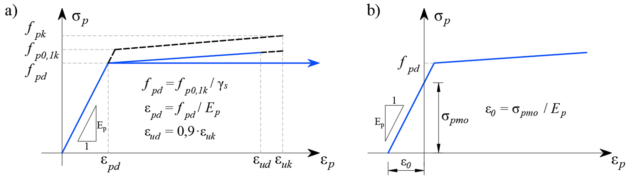
ACI
Spanning-rek diagram van voorspanningswapening: a) Spanning-rek diagram; b) beginrek voor vooraf gespannen wapening

De wapeningselementen zijn via een hechting model verbonden met de 2D elementen van het betonmodel op dezelfde wijze als de klassieke betonwapening.
De hechtingmodelelementen laten de relatieve vervorming van de voorspanningswapening en het beton toe met passende niet-lineaire kenmerken. Dit modelleert correct de aanhechting van de wapening met het beton en ook het verankeringsmodel van de vooraf gespannen wapening. De eindaanpassingen van de wapening met nagerekt staal, zoals de ankerplaat, worden gemodelleerd door een element met een stijfheid die overeenkomt met het anker aan het einde van de voorspanningswapening, en de eindvoorspankracht wordt als een oppervlaktebelasting op het betonmodel aangebracht over een oppervlak ter grootte van de ankerplaat. Het model kan de lokale drieassige spanning in het gebied onder het anker niet correct beschrijven; dit gebied moet afzonderlijk worden beschouwd.
De tension stiffening van de wapening als gevolg van betoninteracties wordt niet in aanmerking genomen bij de voorspanningswapening, omdat het beton in de nabijheid van de voorspanningswapening wordt verondersteld onder druk te staan.
Vooraf gespannen wapening
De vooraf gespannen wapening wordt voorspannen vóór het storten van het element; de voorspanningswapening wordt vrijwel altijd als een rechte lijn geleid, waardoor er geen wrijvingsverliezen optreden. Zodra de vereiste betonsterkte is bereikt, wordt de wapening losgelaten van de ankerblokken, waardoor de voorspanningswapening wordt geactiveerd en de krachten van de wapening naar het beton worden overgedragen. Dit effect is fysisch equivalent aan het onderkoelen van de wapening en wordt gemodelleerd door een beginrek vergelijkbaar met die van thermische belasting. Dit geeft een spanning-rek diagram van voorspanningswapening zoals weergegeven in de bovenstaande figuur onder b). Het rekenmodel berekent automatisch de vervormingsrespons van de constructie op de aangebrachte voorspanning en bepaalt daarmee direct de voorspanningsverliezen door elastische rek van het element.
Omdat de voorspankracht bekend is, en daarmee ook de voorspanningsspanning σpmo, wordt het materiaaldiagram van de wapening gebruikt voor de spanningsafhankelijkheid van de vervorming en kan worden geschreven als:
\[{{σ}_{p}}=~{{f}}({{ε}}-{{ε}_{0}})\]
Ervan uitgaande dat de voorspanning in de wapening lager is dan de vloeigrens (d.w.z. de voorwaarden gedefinieerd in EN 1992-1-1, hoofdstuk 5.10.3 zijn vervuld), kan de beginvervorming ook worden berekend als:
\[{{ε}_{0}}=\frac{{{σ}_{pm0}}}{{{E}_{p}}}\]
ε0 - beginrek door voorspanning
σpm0 - spanning vlak voor loslaten
Ep - elasticiteitsmodulus voor voorspanningswapening
Vooraf gespannen wapening is specifiek doordat de verankering van de uiteinden wordt gerealiseerd door verschillende mechanismen - adhesie van de wapening en het beton op moleculair niveau, de wrijving die ontstaat op het grensvlak tussen het oppervlak van de wapening en het beton, mechanisch indrukken van de spiraalvormige wapening in het beton, en een toename van de diameter van de voorspanningswapening bekend als het wigmechanisme of Hoyer-effect. De bovengenoemde effecten zijn opgenomen in het CSFM rekenmodel door de eigenschappen van het verankeringsmodel in het eindgebied van de vooraf gespannen wapening aan te passen.
Interactie van vooraf gespannen wapening en beton: a) spiraalvormige wapening die in beton drukt; b) Hoyer-effect

Wapening met nagerekt staal
De wapening met nagerekt staal wordt voorspannen nadat de constructie is gestort. Het voorspanningsapparaat wordt direct in de constructie ondersteund, waardoor de verliezen door elastische rek van de constructie door voorspanning worden geëlimineerd. Zodra de gewenste voorspankracht is bereikt, wordt de wapening verankerd en worden de kabelkanalen vervolgens geïnjecteerd, waardoor een hechtingverbinding van de wapening met de constructie wordt bereikt. Bij het modelleren van wapening met nagerekt staal wordt de berekening daarom verdeeld in meerdere belastingstappen - voorspanning, aanbrengen van andere permanente belastingen en aanbrengen van veranderlijke belastingen.
Eindige-elementen betonmesh met gekoppelde 1D voorspanningswapeningselementen:

Belastingstap "voorspanning"
Bij het voorspannen van de wapening wordt de stijfheid van de wapening niet opgenomen in de stijfheid van de constructie. In deze belastingstap wordt de stijfheid van het lineaire element niet in het model beschouwd; de wapeningselementen worden vervangen door een vervangingsbelasting die overeenkomt met de voorspanningsspanning en het wapeningsoppervlak zoals weergegeven in de bovenstaande figuur. Na het bereiken van de volledige belasting door de voorspanning en convergentie van deze belastingstap wordt de vervorming van het specifieke lineaire element afgelezen; op basis van de vervorming wordt de beginrek ε0 van de afzonderlijke lineaire elementen van de voorspanningswapening bepaald.
De voorspanningsspanning kan handmatig worden gedefinieerd over de lengte van de wapening of automatisch worden berekend op basis van de geometrie van de wapening. Als de automatische berekening van verliezen wordt gekozen, worden wrijvingsverlies (volgens EN 1992-1-1, 5.10.5.2, of ACI 318-19, 20.3.2) en wapeningsslip (indrukken van ankerwig) tijdens verankering in aanmerking genomen. Omdat alle voorspanningswapening in één stap wordt aangebracht, wordt verlies door opeenvolgende voorspanning niet beschouwd.
Volgende belastingstappen met ingeschakelde voorspanningswapening
In de volgende belastingstappen (aanbrengen van andere permanente en veranderlijke belastingen) wordt dezelfde procedure gevolgd als voor vooraf gespannen wapening. De volledige stijfheid van de voorspanningswapening wordt beschouwd, de aanhechting tussen de wapening en het omringende beton wordt beschouwd, en het spanning-rek diagram van de voorspanningswapening wordt aangepast door de beginrek ε0. Deze rek is voor elk element verschillend en werd verkregen uit de vorige belastingstap "voorspanning". Door de aanhechting van de wapening en het beton wordt de verandering van voorspanning als gevolg van de elastische vervorming van de constructie door de uitwendige belasting correct in het model beschouwd.
Referenties
ACI Committee 318. 2019. Building Code Requirements for Structural Concrete (ACI 318-19) and Commentary. Farmington Hills, MI: American Concrete Institute.
Alvarez, Manuel. 1998. Einfluss des Verbundverhaltens auf das Verformungsvermögen von Stahlbeton. IBK Bericht 236. Basel: Institut für Baustatik und Konstruktion, ETH Zurich, Birkhäuser Verlag.
Beeby, A. W. 1979. "The Prediction of Crack Widths in Hardened Concrete." The Structural Engineer 57A (1): 9–17.
Broms, Bengt B. 1965. "Crack Width and Crack Spacing In Reinforced Concrete Members." ACI Journal Proceedings 62 (10): 1237–56. https://doi.org/10.14359/7742.
Burns, C.. 2012. "Serviceability Analysis of Reinforced Concrete Members Based on the Tension Chord Model." IBK Report Nr. 342, Zurich, Switzerland: ETH Zurich.
Crisfield, M. A. 1997. Non-Linear Finite Element Analysis of Solids and Structures. Wiley.
European Committee for Standardization (CEN). 2015. 1 Eurocode 2: Design of concrete structures - Part 1-1: General rules and rules for buildings. Brussels: CEN, 2005.
Fernández Ruiz, M., and A. Muttoni. 2007. "On Development of Suitable Stress Fields for Structural Concrete." ACI Structural Journal 104 (4): 495–502.
Kaufmann, W., J. Mata-Falcón, M. Weber, T. Galkovski, D. Thong Tran, J. Kabelac, M. Konecny, J. Navratil, M. Cihal, and P. Komarkova. 2020. "Compatible Stress Field Design Of Structural Concrete. Berlin, Germany."AZ Druck und Datentechnik GmbH, ISBN 978-3-906916-95-8.
Kaufmann, W., and P. Marti. 1998. "Structural Concrete: Cracked Membrane Model." Journal of Structural Engineering 124 (12): 1467–75. https://doi.org/10.1061/(ASCE)0733-9445(1998)124:12(1467).
Kaufmann, W.. 1998. "Strength and Deformations of Structural Concrete Subjected to In-Plane Shear and Normal Forces." Doctoral dissertation, Basel: Institut für Baustatik und Konstruktion, ETH Zürich. https://doi.org/10.1007/978-3-0348-7612-4.
Konečný, M., J. Kabeláč, and J. Navrátil. 2017. Use of Topology Optimization in Concrete Reinforcement Design. 24. Czech Concrete Days (2017). ČBS ČSSI. https://resources.ideastatica.com/Content/06_Detail/Verification/Articles/Topology_optimization_US.pdf.
Marti, P. 1985. "Truss Models in Detailing." Concrete International 7 (12): 66–73.
Marti, P. 2013. Theory of Structures: Fundamentals, Framed Structures, Plates and Shells. First edition. Berlin, Germany: Wiley Ernst & Sohn.
http://sfx.ethz.ch/sfx_locater?sid=ALEPH:EBI01&genre=book&isbn=9783433029916.
Marti, P., M.Alvarez, W. Kaufmann, and V. Sigrist. 1998. "Tension Chord Model for Structural Concrete." Structural Engineering International 8 (4): 287–298.
https://doi.org/10.2749/101686698780488875.
Mata-Falcón, J. 2015. "Serviceability and Ultimate Behaviour of Dapped-End Beams (In Spanish: Estudio Del Comportamiento En Servicio y Rotura de Los Apoyos a Media Madera)." PhD thesis, Valencia: Universitat Politècnica de València.
Meier, H. 1983. "Berücksichtigung Des Wirklichkeitsnahen Werkstoffverhaltens Beim Standsicherheitsnachweis Turmartiger Stahlbetonbauwerke." Institut für Massivbau, Universität Stuttgart.
Navrátil, J., P. Ševčík, L. Michalčík, P. Foltyn, and J. Kabeláč. 2017. A Solution for Walls and Details of Concrete Structures. 24. Czech Concrete Days.
Schlaich, J., K. Schäfer, and M. Jennewein. 1987a. "Toward a Consistent Design of Structural Concrete." PCI Journal 32 (3): 74–150.
Standards Australia. 2018. Concrete Structures (AS 3600:2018). Sydney, NSW: Standards Australia.
Standards Australia. 2022. Concrete Structures – Commentary (Supplement 1 to AS 3600:2018). Sydney, NSW: Standards Australia.
Vecchio, F.J., and M.P. Collins. 1986. "The Modified Compression Field Theory for Reinforced Concrete Elements Subjected to Shear." ACI Journal 83 (2): 219–31.